11.3: Amplifiers

Last updated
Save as PDF

Page ID: 41337

\( \newcommand{\vecs}[1]{\overset { \scriptstyle \rightharpoonup} {\mathbf{#1}} } \) \( \newcommand{\vecd}[1]{\overset{-\!-\!\rightharpoonup}{\vphantom{a}\smash {#1}}} \)\(\newcommand{\id}{\mathrm{id}}\) \( \newcommand{\Span}{\mathrm{span}}\) \( \newcommand{\kernel}{\mathrm{null}\,}\) \( \newcommand{\range}{\mathrm{range}\,}\) \( \newcommand{\RealPart}{\mathrm{Re}}\) \( \newcommand{\ImaginaryPart}{\mathrm{Im}}\) \( \newcommand{\Argument}{\mathrm{Arg}}\) \( \newcommand{\norm}[1]{\| #1 \|}\) \( \newcommand{\inner}[2]{\langle #1, #2 \rangle}\) \( \newcommand{\Span}{\mathrm{span}}\) \(\newcommand{\id}{\mathrm{id}}\) \( \newcommand{\Span}{\mathrm{span}}\) \( \newcommand{\kernel}{\mathrm{null}\,}\) \( \newcommand{\range}{\mathrm{range}\,}\) \( \newcommand{\RealPart}{\mathrm{Re}}\) \( \newcommand{\ImaginaryPart}{\mathrm{Im}}\) \( \newcommand{\Argument}{\mathrm{Arg}}\) \( \newcommand{\norm}[1]{\| #1 \|}\) \( \newcommand{\inner}[2]{\langle #1, #2 \rangle}\) \( \newcommand{\Span}{\mathrm{span}}\)\(\newcommand{\AA}{\unicode[.8,0]{x212B}}\)

Amplifier modules must be optimized for low noise, moderate to high gain, high efficiency, stability, low distortion, and particular output power. Usually

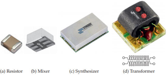
Figure \(\PageIndex{1}\): Modules in surface-mount packages. Copyright Synergy Microwave Corporation, used with permission [1].

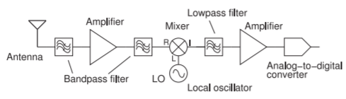
Figure \(\PageIndex{2}\): Receiver as a cascade of modules.

an application note provided by the amplifier module vendor indicates how to do this for their module. Amplifiers require input and output matching networks as shown in Figure \(\PageIndex{5}\). The DC bias control circuit is fairly standard and the lowpass filters (in the bias circuits) are often incorporated into the input and output matching networks. Manufacturers of amplifier modules provide substantial information, including \(S\) parameters and, in many cases, reference designs.

Some amplifier modules come with input and output matching networks embodied in the module package. Since matching networks have limited bandwidth, incorporating them in the module sets the operating frequency range. Alternatively the designer can design the input and output matching networks and thus control the operating frequency.

Usually the module manufacturer provides a reference design and often

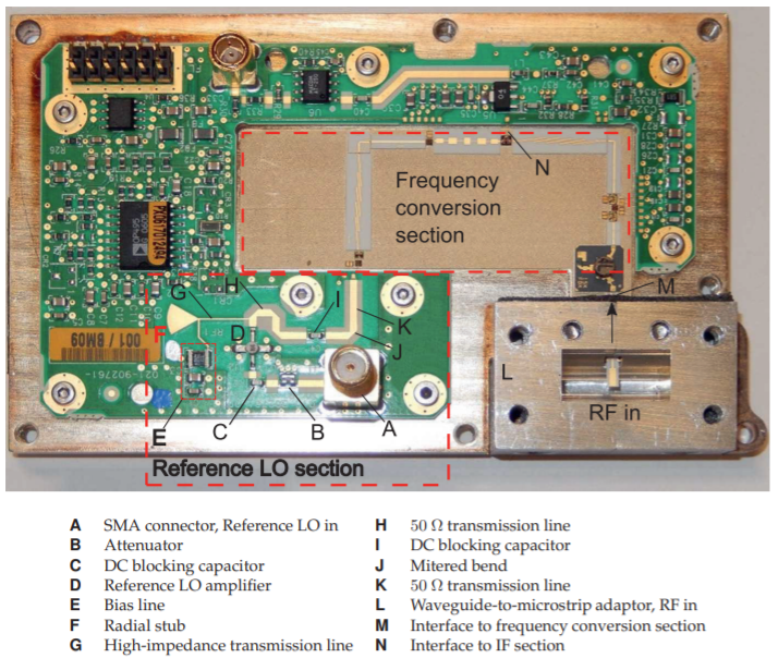
Figure \(\PageIndex{3}\): A \(14.4–15.35\text{ GHz}\) receiver consisting of cascaded modules interconnected by microstrip lines. Surrounding the microwave circuit are DC conditioning and control circuitry. RF in is \(14.4\text{ GHz}\) to \(15.35\text{ GHz}\), LO in is \(1600.625\text{ MHz}\) to \(1741.875\text{ MHz}\). The frequency of the IF is \(70–1595\text{ MHz}\). Detail of the frequency conversion section is shown in Figure \(\PageIndex{4}\).

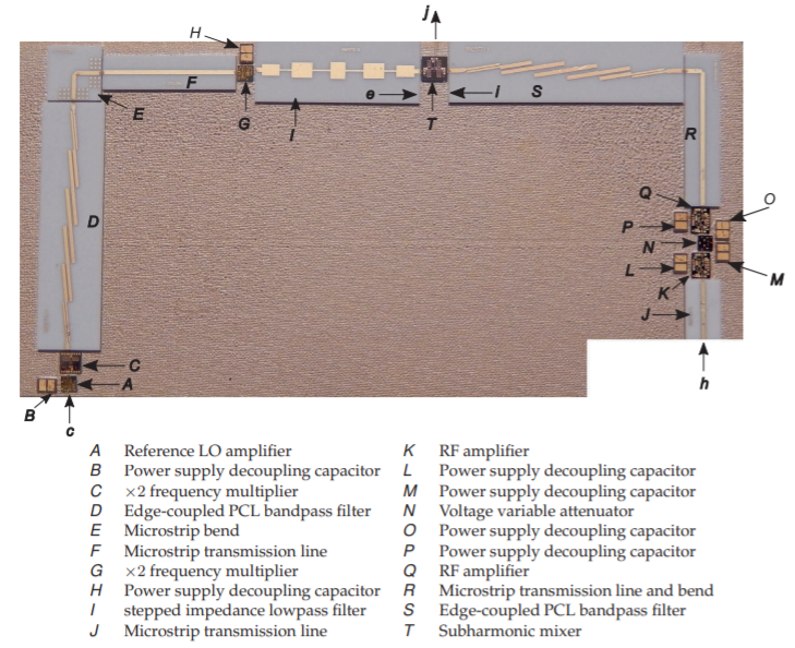
Figure \(\PageIndex{4}\): Frequency conversion section of the receiver module. The reference LO is applied at \(\mathsf{c}\), the RF is applied at \(\mathsf{h}\) following the isolator. The IF is output at \(\mathsf{j}\).

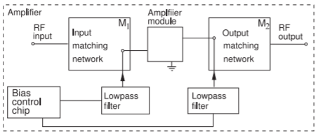
Figure \(\PageIndex{5}\): Block diagram of an RF amplifier including biasing networks.

an evaluation board, e.g. see the evaluation board in Figure \(\PageIndex{6}\) for a power amplifier. This module does not include input and output matching networks but these are provided on the evaluation board.

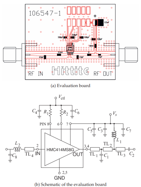
Figure \(\PageIndex{6}\): Evaluation board for the HMC414MS8G GaAs InGaP HBT MMIC power amplifier module operating between \(2.2\) and \(2.8\text{ GHz}\). The amplifier provides \(20\text{ dB}\) of gain and \(+30\text{ dBm}\) of saturated power at \(32\%\) PAE from a \(+5\text{ V}\) supply voltage. The amplifier can also operate with a \(3.6\text{ V}\) supply selectable by the resistors \(R_{1}\) and \(R_{2}\). Copyright Hittite Microwave Corporation, used with permission [2].