4.1: Procedure

In previous work we have examined the basic functionality of TINA, namely basic schematic capture functions such as component selection, placement, and parameter editing, along with simple simulations using voltmeters and the nodal voltages probe to measure DC voltage. While this method is relatively quick and easy to use, it is limited in other aspects. Some of the issues include:

1. Limited measurements per unit, for example a single measurement for a voltmeter, requiring multiple units for multiple measurements.

2. The need to rewire the instruments (and hence the schematic) in order to take different readings.

3. Excessive amount of work space area obscured by the instrument(s) with accompanying clutter.

4. No convenient way of storing and recalling prior simulations.

5. No convenient means of exporting simulated measurement data to other programs.

To address these issues TINA allows for an all-in-one analysis using a Table of Results and also a graphing window. Large amounts of data may be displayed simultaneously. These data may also be saved as a text file for later examination or for input into other programs.

Nothing “extra” needs to be added to the circuit. Instead of choosing the DC Analysis->Calculate nodal voltages menu item, instead, select the DC Analysis->Table of DC results menu item. To illustrate, begin by building the circuit shown in Figure \(\PageIndex{1}\). Drag a DC voltage source, an earth ground and two resistors onto the work space. Connect them in a series loop and edit the component values to 20 volts for the source, and 4000 and 6000 ohms for the two resistors.

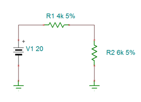
Figure \(\PageIndex{1}\)

Notice that no voltmeters are required. From the Analysis menu, select DC Analysis->Table of DC results, as shown in Figure \(\PageIndex{2}\).

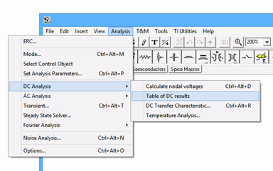
Figure \(\PageIndex{2}\)

In a moment, the Table of Results window will open as shown in Figure \(\PageIndex{3}\). You may need to enlarge the window in order to see all of the values.

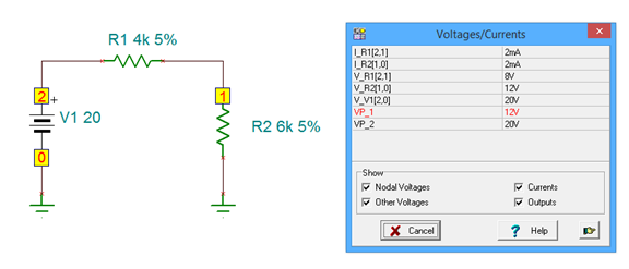
Figure \(\PageIndex{3}\)

This window lists all of the component voltages and currents in the circuit. Essentially, it's like using the probe on everything and then collecting all of the data in one place. This list can be saved as a text file by selecting the small “finger point” button in the lower right. All values are identified by the component's name. You will also notice that every connection point in the circuit has been given a number. Ground is always 0 and the remaining points are sequentially numbered as the circuit is wired together. Note that voltage points 1 and 2 (VP_1 and VP_2) are included in the list and that each component's current or voltage is also identified by these numbers. For example, the voltage across resistor R1 is identified as V_R1[2,1]. The [2,1] indicates that the component is connected from node 2 to node 1. The first number is the connection for the positive lead of the meter while the second is the connection for the negative lead. Thus, this indicates the polarity and direction of the voltage and current.

It is worth noting that although TINA also has an ammeter similar to its voltmeter, this method tends to be much more efficient for current measurement because ammeters must be inserted in series with the component of interest. That is, the circuit must be rewired to accommodate the ammeter, unlike a voltmeter which is simply placed across the component(s) of interest.

At this point, you might be wondering why you would ever not use this method, abandoning the original method and voltmeters entirely. There are two cases where using the original method and/or voltmeters may be preferred. First, in very large circuits the table of values can be overwhelming. Second, as is, there is no obvious way of determining a voltage that appears across several components, short of adding up the individual voltages manually. In this case, a voltmeter can still be used, its value will show up in the table alongside the other component voltages.

Finally, you may prefer to give the connection points names, such as Vin or node A, instead of the default numbering scheme. This can be achieved by adding Voltage Pins to the schematic. This is the first item in the Meters tab and looks like the letter C with a tail. These items can be placed anywhere on a schematic, and once added, the names can be changed. This is illustrated in Figure \(\PageIndex{4}\). Two voltage pins have been added to the locations formerly known as nodes 1 and 2. The names have been changed to “b” and “a”, respectively. Note that the table of voltages and currents now uses these letters instead of the numbers.

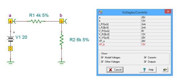
Figure \(\PageIndex{4}\)

Finally, the table still makes use of the mouse probe. If you click on a Voltage Pin, its entry will be highlighted in the table. If you click on a component, the entries for both its current and voltage will be highlighted.

There are times when graphical data is preferred over simple numeric data. To illustrate this, we will shift our attention to time domain waveform analysis using an AC source. To do this, first delete the DC source in your existing circuit. Replace it with an AC voltage generator. This is the fourth item in the Sources tab. Your circuit should like similar to the one shown in Figure \(\PageIndex{5}\).

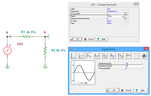
Figure \(\PageIndex{5}\)

The AC generator is very flexible. We would like to create a 20 volt peak sine wave at a frequency of 1 kHz. To do this, double click on the generator to open its settings dialog box. Click on the Signal row to reveal a small ellipsis button (…). Clicking on the ellipsis brings up the Signal Editor. Select the sine shape (third item) and set the Amplitude to 20 and the frequency to 1000 Hz (1k, for short). Select OK for both of these windows.

From the Analysis menu, select Transient. The Transient Analysis dialog opens, as shown in Figure \(\PageIndex{6}\).

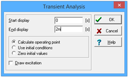
Figure \(\PageIndex{6}\)

We would like to see the first two milliseconds of our waveform. At 1 kHz, we should see two full cycles. Enter a start time of 0 and and end time of 2m (0.002 seconds). After selecting OK, a graphing window opens as shown in Figure \(\PageIndex{7}\). Notice that the time scale runs from 0 to 2 milliseconds and the amplitude spans from -20 to +20 volts. Two waveforms are drawn, node voltages \(a\) and \(b\), as requested by our Voltage Pins.

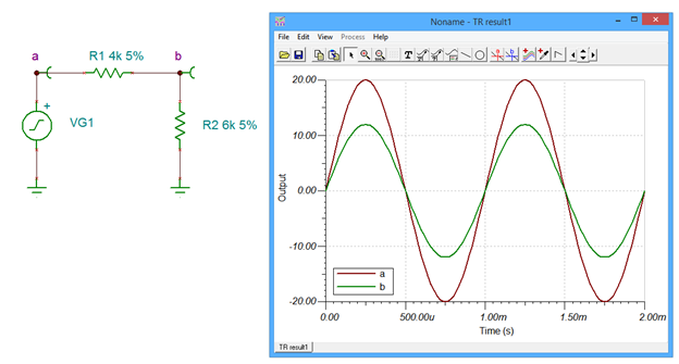
Figure \(\PageIndex{7}\)

There are several useful tools and variations you can utilize with this graphing window. They are accessed either through the menus or the toolbar. For example, you can zoom into any part of the wave for closer inspection by using the zoom tool (magnifying glass). For precise measurements of the waveforms, you can make use of the cursors. There are two cursors labeled \(a\) and \(b\) (red and blue crosses in the toolbar). To use a cursor, select the cursor button and then hover the mouse over the waveform of interest. The mouse pointer will change shape into a cross. Click on the waveform. This will produce a pair of horizontal and vertical lines that track the waveform. You can move the cursor by grabbing the associated letter tab at the top of the graph with the mouse. The values at the intersection are displayed in a small output window. If both cursors are active, the output window will also include the differences between the two sets of cursor values. This is illustrated in Figure \(\PageIndex{8}\) where the the bottom line displays the difference in the horizontal X values (here, that's time), and the vertical Y values (in this case, voltage).

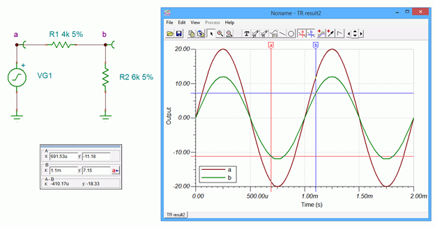
Figure \(\PageIndex{8}\)

You may wish to separate the curves instead of displaying them together. This can be achieved through the View menu options Separate/Collect curves, as shown in Figure \(\PageIndex{9}\).

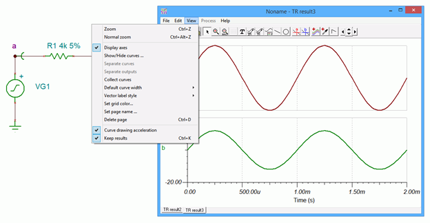
Figure \(\PageIndex{9}\)

Some other graph attributes can be modified through the View menu such as the color of the grid and the visibility of the axes. Double clicking on a curve will allow you to set the color of the curve, its thickness and other characteristics. Unique labels can be applied using the Text tool (capital T on the toolbar and essentially the same as the one found in the main program toolbar). A pointer can be added to the text with the use of the Text Pointer button (a small T with an arrow). The horizontal and vertical axes can be formatted by double clicking on them. This will bring up the Set Axis dialog box. Here you can change the label, set the numeric format and precision, and also set the scale range and type. This is illustrated in Figure \(\PageIndex{10}\).

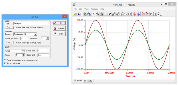
Figure \(\PageIndex{10}\)

One particularly interesting toolbar button is the one immediately to the right of the cursors. This is the Post Processor. Selecting this will allow you to create complex expressions that can then be plotted. For example, you might wish to find the difference between two voltages or the current through a section of a circuit by dividing its voltage curve by the associated resistance.

The process is fairly straightforward. The Post Processor dialog is illustrated in Figure \(\PageIndex{11}\). On the left is a list of available signals. In this example we have the voltages from node a to ground and from node b to ground. Suppose we would like to plot the voltage seen across R1. This is voltage \(a\) minus voltage \(b\). Select a from the list and copy it to the Line Editor by clicking on the large downward arrow. Now, select the minus sign from the drop down list of built-in functions and copy this down to the Line Editor. Finally, select \(b\) from the curves list and copy it down.

We now have an expression to plot. It can be previewed with the Preview button before selecting OK. This curve is shown in bright blue in the graphing window.

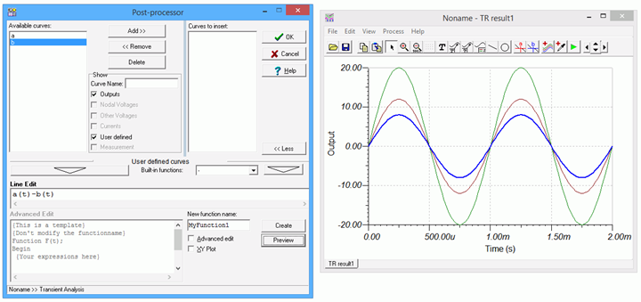
Figure \(\PageIndex{11}\)