1.2: Atomic Structure

In our effort to understand the operation of semiconductors, a fundamental question we might ask is “What is the internal structure of an atom?” Please understand that it is nonsensical to ask what an atom might “look like” because its components are all smaller than the shortest wavelengths of light that humans can see. Instead, we simply need a model to explain its observed behavior.

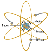
Figure \(\PageIndex{1}\): Planetary atomic model: Pretty, well-known and wrong. Image source (modified)

Perhaps the most prolific model in the popular imagination is the planetary model shown in Figure \(\PageIndex{1}\). In this model, the core, or nucleus, is drawn at the center and contains positively charged protons and non-charged neutrons. Revolving around this core are negatively charged electrons, each following a nice, regular, planar path much like a planet around the sun. Unfortunately for us, this model is starkly incorrect, although it has found use as a symbol for nuclear regulatory agencies and a DEVO album cover from the 1970s.

Before we come up with a more accurate and useful model, let's take a closer look at the sub-components; namely the proton, neutron and electron. First off, most of the mass of any given atom is from the protons and neutrons. Protons and neutrons have similar masses, about 1.67E−24 grams each. The mass of an electron is roughly 2000 times smaller. The radius of a proton is approximately 0.87E−15 meters and the mean distance to the nearest electron is about 5.3E−11 meters. This means that this electron is about 60,000 times farther away from the proton than the size of said proton. To put this into perspective, that's roughly the same as the ratio between a golf ball and a sphere with a radius of 3/4ths of a mile or 1200 meters. This would be the case for a hydrogen atom as it consists of a single proton and electron. The magnitude of this ratio is not much different for other substances, including things like crystalline carbon (diamond) and quartz (a molecule of silicon and oxygen) that are very hard and solid. If you think about that for a moment, you realize that the idea of “solidity” is in some ways an illusion because the vast majority of what we call “something” is really just empty space. For example, chances are that you are sitting down while reading this. You probably feel your buttocks pressed against the chair. Both of these things are considered solid yet at the atomic level the vast majority of both items is nothingness. In reality, the feeling of solidity is just the result of the interaction of atomic forces between the two. So if someone suggests that you might have a bit too much to spare in the department of the posterior, you can inform them that it's really nothing.

One of the major issues with the planetary model is the idea that electrons whirl around the nucleus in stable, planet-like orbits. That's simply not true. First, the electron inhabits a region of 3D space, it does not simply move through a plane. Second, due to the Heisenberg Uncertainty Principle, we can't precisely plot the position and trajectory of a given electron. The best we can do is make a plot of where the electron is likely to be. This is called a probability contour. Imagine that you could record the position of an electron relative to the nucleus. A moment later you record its new position, a moment after that you record the next position, and on and on for thousands of measurements. If you attempted to plot them all, you would wind up with a cloud of dots around the nucleus. This cloud is referred to as an orbital. You wouldn't know how the electron got from one position to the next but you would get a general idea of where it was likely to be. Do not confuse orbital with orbit (like a planetary orbit). They are two different beasties.

There are several potential orbitals. Due to quantum physics, only certain orbitals are allowed. The permissible electron energy levels are first grouped into shells, then subshells and finally orbitals. It is important to remember that orbitals indicate the electron energy level. That is, a higher orbital implies a higher energy level. Further, orbitals fill in first from lowest energy level to highest energy level. These are important ideas that we will leverage in future discussions.

Shells are denoted by their principal quantum number, \(n\); 1, 2, 3, etc. The higher the number, the more subshells it can contain. Subshells are organized by their orbital shape and are designated by letters, the first four being \(s\), \(p\), \(d\), and \(f\). Shell 1 contains only subshell \(s\) while shell 2 contains subshell types \(s\) and \(p\). Shell 3 contains subshell types \(s\), \(p\) and \(d\), and so on.

Thus, we see designations such as \(1s\), \(2s\) and \(2p\). These subshells may also have variations within them. There is one variation on \(s\), three variations on \(p\), five variations on \(d\), etc. These variations are the orbitals and each orbital can hold a maximum of two electrons.

Putting this all together, we find that the first shell can contain a maximum of two electrons: two in the single \(s\) subshell orbital (\(1s\)). The second shell can contain a maximum of eight electrons: two in the \(s\) subshell (\(2s\)) plus two in each of the three \(p\) subshell orbitals (\(2p\)). In like manner the third shell can contain a maximum of 18 electrons: two in \(3s\), six in \(3p\) and two in each of the the five \(d\) subshell orbitals (\(3d\)). You can condense this into a simple formula, \(2n^2\), where \(n\) is the shell number.

Figure \(\PageIndex{2}\): Electron probability contour for innermost orbital, \(1s\). Image source

Figure \(\PageIndex{2}\) shows the electron probability contour of the innermost orbital, namely \(1s\) (i.e., principle quantum number 1, subshell \(s\)). As you can see, it is spherical in shape. The nucleus is located at the center, obscured here. All \(s\) orbitals are similarly spherically shaped although the internals change. \(1s\) is the lowest energy orbital.

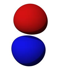
Figure \(\PageIndex{3}\): Electron probability contour for orbital \(2p\). Image source

Orbitals are not limited to simple spherical shapes. Higher order orbitals can take on a variety of forms. Figure \(\PageIndex{3}\) shows the electron probability contour for the \(2p\) orbitals (recall there are three \(p\) variations, one each oriented along the X, Y and Z axes). The nucleus is situated in the small void between the two lobes. Obviously, this is nothing like the well-behaved elliptical orbits of planets around the sun. Probability contours can be very complex. For the highest orbitals, especially when combined with the lower orbitals, the contour combinations can become reminiscent of the sculptures of a deranged clown forming herds of imaginary balloon animals.

As interesting as these graphics are, they are cumbersome to work with. Consequently, a more functional graphic is called for. Such a device is the Bohr model, named after Danish physicist Niels Bohr. An example is shown in Figure \(\PageIndex{4}\).

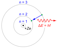
Figure \(\PageIndex{4}\): Generic Bohr model. Image source

It is important to understand that the Bohr model is an energy description of the atom, not an attempt to mimic its physical appearance or structure. The nucleus is placed at the center. It is surrounded by concentric rings that represent the electron shells. The higher the number, the larger the ring and the greater the energy level. If an electron were to move from a higher level to a lower level, the energy difference is radiated out. This could be in the form of heat or light. This is a point worth remembering. For example, this transition is what makes light emitting diodes (LEDs) function. The inverse is also possible, namely that by absorbing energy, an electron can move into a higher orbital. This is an equally powerful concept, as we shall soon see.

Using the Bohr model we can create diagrams to represent individual elements. For example, copper has an atomic number of 29 meaning that it has 29 protons and 29 electrons. The electron shell configuration is 2-8-18-1. That is, the first three shells are completely filled and there is a single electron in the fourth shell. This single outer electron is only loosely bound and thus makes copper a very good conductor. The Bohr model for copper would simply show four rings, the first three being filled and with a single electron in the fourth ring.

Figure \(\PageIndex{5}\) shows the Bohr model of an atom of Silicon, atomic number 14, with an electron shell configuration of 2-8-4. In this version, the individual electrons are drawn in each shell and the atomic number is indicated at the nucleus. Again, please do not imagine this representing individual electrons orbiting the nucleus in lanes. This is an energy level depiction.

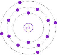
Figure \(\PageIndex{5}\): Bohr model of Silicon.

Often, it is useful to simplify this model further by omitting the filled inner shells. Also, the atomic number is replaced by the number of electrons in the outermost, or valence, shell. This is shown in Figure \(\PageIndex{6}\). The valence shell is particularly important as it gives insight into the general behavior of the material.

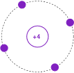
Figure \(\PageIndex{6}\): Simplified Bohr model of Silicon.

As an alternative, sometimes we will “straighten out” the Bohr model so that it simply shows the energy levels graphically as lines or bands, and without counting specific electrons. This is depicted in Figure \(\PageIndex{7}\).

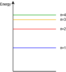
Figure \(\PageIndex{7}\): Energy level diagram.