8.4: Loudspeakers

One of the more common loads for amplifiers is a loudspeaker. It makes sense then to look at how they are constructed and note anything interesting or peculiar as far as their electrical characteristics are concerned. The most common form of loudspeaker is the dynamic loudspeaker¹. All dynamic loudspeakers share certain common elements regardless of size or acoustic output capability. A cutaway view of a low frequency driver is shown in Figure \(\PageIndex{1}\).

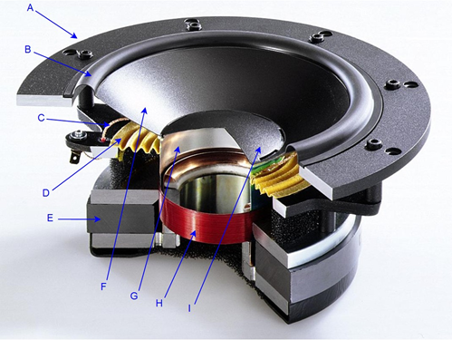
Figure \(\PageIndex{1}\): Dynamic loudspeaker. A. Frame B. Suspension C. Lead wire D. Spider E. Magnet F. Diaphragm G. Voice coil former H. Voice coil I. Dust cap Image courtesy of Audio Technology

The idea behind its operation is magnetic repulsion and attraction. The heart of the unit is the voice coil (H). This is a coil of magnet wire wound around a former (G) that typically is made of aluminum or some other high temperature material. The voice coil might be a single layer of edge-wound ribbon wire or perhaps several layers of ordinary round wire. Depending on the design, the voice coil might be anywhere from a fraction of an inch to several inches in diameter. The coil ends are connected to flexible lead wires (C) that terminate on the loudspeaker frame (A). Ultimately, that's what the amplifier will connect to.

The voice coil is fixed to a diaphragm (F) and is freely suspended by an outer edge suspension (B) and an inner element known as a spider (D). The voice coil sits in a strong magnetic field that is created by a powerful permanent magnet (E) that commonly uses ceramic, alnico or rare earth construction. When current from the amplifier flows through the coil, it will create it's own magnetic field that will either aid or oppose the fixed field created by the permanent magnet, depending on the direction of the current. This results in a force that causes the coil to move within the fixed field. As the coil moves, the diaphragm moves with it, pushing on the surrounding air and creating sound. The larger the current, the stronger the newly created field and the greater the resulting aid or opposition, which results in greater movement of the diaphragm and a larger sound pressure. This fundamental design has changed little since its invention in the 1920s. Modern magnets, suspension and diaphragm materials have improved considerably in the intervening years but the operational principle is pretty much the same.

It is very difficult to create a driver that can cover the full audio spectrum of 20 Hz to 20 kHz while achieving sufficient listening volume at low distortion. Consequently, drivers are often designed to cover a limited portion of the audio spectrum. Low frequency drivers are commonly referred to as woofers while high frequency drivers are called tweeters. Drivers that cover the middle range of frequencies are given the highly inventive name midranges (although once upon a time they were called squawkers). A combination of these devices will be wired together with other components to create a complete home or auto loudspeaker system. Although very high quality systems can be produced, virtually all direct radiating dynamic loudspeaker systems suffer from low conversion efficiency. For a typical consumer system, only about 1% to 2% of the applied electrical power is turned into useful acoustic output power. The vast majority of the applied power simply makes the voice coil hot.

8.4.1: Loudspeaker Impedance

Loudspeakers are given a nominal impedance value. The most common impedance for home use is 8 \(\Omega\) while 4 \(\Omega\) is common in automotive systems. It is important to remember that this is a nominal value and the true value varies with frequency. While it is common to test power amplifiers with large power resistors, they are only a coarse approximation of a real loudspeaker.

The electrical and mechanical characteristics of a loudspeaker combine to create an equivalent circuit with resistive, inductive and capacitive elements. A typical electrical circuit model² of a single loudspeaker driver is shown in Figure \(\PageIndex{2}\). \(R_{VC}\) and \(L_{VC}\) are the resistance and inductance of the voice coil, respectively. The other components are electrical equivalents of mechanical properties such as suspension losses.

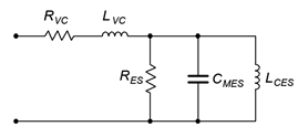
Figure \(\PageIndex{2}\): Dynamic loudspeaker electrical model.

Clearly, this is not a simple 8 \(\Omega\) resistor. In fact, we see a very complex impedance: The three parallel elements will create a resonant peak and the series inductance will cause the impedance to rise with frequency. Typically, the resonant peak occurs at the lower end of the spectrum and the associated resonant frequency is denoted on a spec sheet as \(f_S\), the free-air resonance. For a nominal 8 \(\Omega\) woofer, the peak impedance can be over 30 \(\Omega\). An example of a loudspeaker impedance plot is shown in Figure \(\PageIndex{3}\).

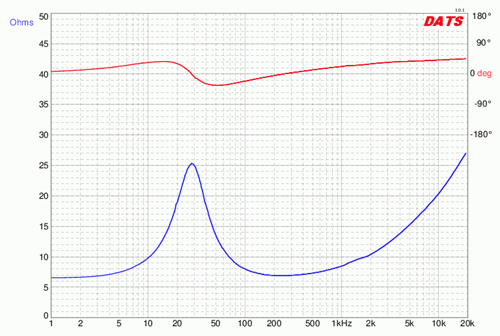
Figure \(\PageIndex{3}\): Dynamic loudspeaker impedance plot. Courtesy of Dayton Audio.

This loudspeaker is a nominal 8 \(\Omega\) unit yet the impedance can be many times this value, and at some frequencies, less than 7 \(\Omega\). This plot also includes the phase angle of the loudspeaker and we can see that it can be upwards of 40\(^{\circ}\) capacitive or inductive, depending on the frequency. What makes this more interesting is that a consumer loudspeaker system is a combination of multiple drivers plus other electrical components, and this can result in an even more complex impedance plot.

The obvious question is, “Does this have any effect on the analysis of the power amplifier?” The simple answer is, “Yes”. Areas of the spectrum where the impedance magnitude drops below the nominal value will require more current for any given load voltage. Further, the phase shift caused by a partly reactive load will impact the power dissipation of the transistor.

Consider the power graph shown in Figure 8.3.6 for a purely resistive load. If we repeat the plot but add a noticeable phase shift to simulate a partly reactive load, something interesting happens, as shown in Figure \(\PageIndex{4}\).

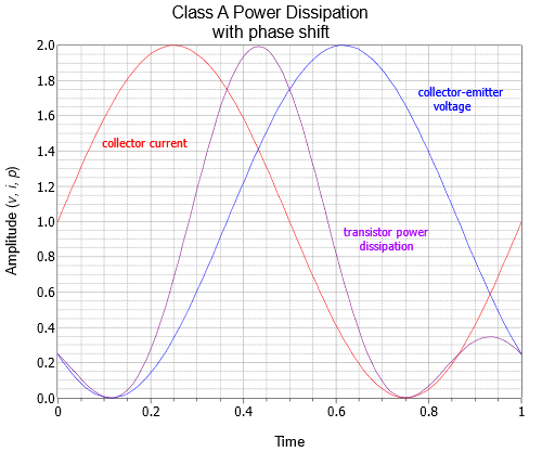
Figure \(\PageIndex{4}\): Power dissipation with reactive load.

The purple trace represents the power dissipation of the transistor. The peak current-voltage product is twice the value seen with a purely resistive load. This combination might lay outside the safe operating area of the transistor. Ultimately, reactive loads are somewhat more “challenging” than simple resistive loads. Therefore, the transistors may need to be rated higher than the values computed for an idealized resistive load.

Another way of looking at the issue of phase shift induced by loudspeakers and other complex loads is to examine the AC load line. Our previous work with load lines always assumed that the load was purely resistive. What happens in the complex impedance case?

If we examine a generic complex load at a single frequency, our former straight line load line turns into an ellipse, as shown in Figure \(\PageIndex{5}\).

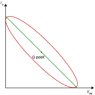
Figure \(\PageIndex{5}\): AC load line with complex load.

This plot assumes that the circuit has a centered Q point. The normal resistive load line is shown in green. We can visualize the signal starting at zero amplitude, meaning all we see is the Q point. As the signal gets larger and larger, it swings along the green line until, eventually, it maxes out at the two axes. In the complex impedance case, we also start at the Q point. As the signal increases, it traces out an ellipse around the Q point. Further increases would create a larger ellipse, and then a larger ellipse, and so on. Eventually, we would see the maximum swing just touching the axes. This is what is plotted above in red, the maximum case (i.e., at full compliance).

If the impedance angle changes, the aspect ratio of the ellipse changes in reaction to it. The larger the angle, the more open the ellipse becomes. The extremes are 0\(^{\circ}\), the purely resistive case that yields a collapsed ellipse or straight line; and 90\(^{\circ}\), the purely reactive case that yields a fully open ellipse, or circle. We have already seen that the phase angle of a loudspeaker changes with frequency, therefore, the load line also changes with frequency. As we sweep the input frequency from low to high, we can imagine the load line wavering back and forth between straight lines and various elliptical shapes. The important thing, though, is that some of these new operating regions (the areas where the red curve is above and to the right of the green line) may go outside the safe operating area of the transistor.

References

¹It's a rather odd name given that all loudspeakers are dynamic in some respect. If they weren't they wouldn't produce sound.

²Adapted from R. H. Small, “Direct Radiator Loudspeaker System Analysis”, Journal of the Audio Engineering Society, June, 1972.