14.3: Pulse Width Modulation

Clearly, class D presents the possibility of minimal wasted power and high efficiency. We are now left with the problem of how to turn a series of pulses into a continuous, smoothly varying waveform, such as a voice or music signal. There are a few ways to accomplish this; it's a matter of encoding the amplitude of the original signal into the pulse train that drives the output devices. Theoretically, as long as the “area under the curve” for a segment of input signal is identical to the area represented by the pulse train, we will have successfully encoded the signal and we then should be able to decode it, turning it back into a smoothly varying output signal. For this to work properly, the pulse train will have to be at much higher frequency than the input signal in order to follow its changes over time. One way to do this is through pulse density modulation, or PDM. The idea is to produce a number of narrow pulses to represent the area. If the input amplitude is large, we create a large number of pulses and if the amplitude is small, we produce a small number of pulses. While this technique can work, it is somewhat challenging to turn this pulse train back into the desired signal at the load.

Another technique to encode the input is pulse width modulation, or PWM. Instead of altering the number of pulses in a given period of time, we keep the frequency constant and adjust the width of the pulses. If the input amplitude is high, the width of the corresponding pulse will be wide and if the amplitude is low, the pulse width will be narrow. The decoding of PWM is easier than that of PDM and is generally the preferred route.

Generating PWM is a relatively straightforward affair. All we need is a triangle wave and a comparator. The comparator has two input terminals: the signal to be encoded (input signal) and the reference wave (triangle wave). It has a two-state, logical output. The output will be high if the signal is more positive than the reference and it will be low if the reference is more positive than the signal. This is shown in block diagram form in Figure \(\PageIndex{1}\).

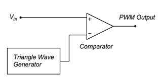
Figure \(\PageIndex{1}\): PWM encoder.

As mentioned, the triangle wave needs to be at a much higher frequency than the signal that is being encoded. As a general rule, this frequency should be at least ten times the highest input signal frequency.

\[f_{triangle} \geq 10 f_2 \label{14.1} \]

A simulation showing the PWM waveforms is presented in Figure \(\PageIndex{2}\).

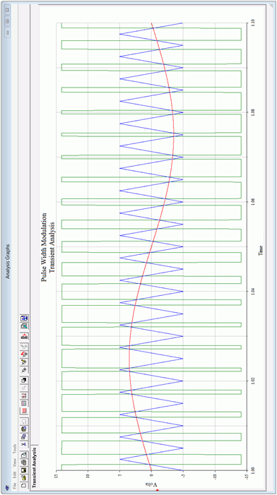
Figure \(\PageIndex{2}\): PWM waveforms.

The input signal is the red sine wave. The blue triangle wave is the reference and is approximately 20 times higher in frequency. The green wave is the PWM output. Note that when the red input signal climbs above the blue reference triangle, the green output goes high, otherwise, the output is low. Thus, the duty cycle of the pulses correlates with the input signal amplitude. The input signal should not exceed the amplitude of the triangle wave otherwise accuracy will impaired. Also, the accuracy of the encoding process is dependent on the linearity of the triangle wave, so a high quality triangle wave generator is needed. Lastly, for accuracy and ease of decoding, the output pulses should not be allowed to become too thin, so the input signal should be limited to about 75% of the amplitude of the triangle wave.

14.3.1: Reconstituting the Output

Although we have successfully encoded the input signal into a series of pulses, we still need to decode them, that is, reconstitute the original continuously variable input signal. Mathematically, the PWM signal contains all of the original input signal frequency components and amplitudes, it just has added a large of number of new frequency components. These new components are multiples (harmonics) of the fundamental PWM frequency, and consequently, they are all higher than the input signal frequencies. As such, they may be removed with a low-pass filter. This will effectively reconstitute the original signal (but at a much higher amplitude, of course). A simple passive \(LC\) filter would be appropriate in this instance as it must pass large currents and voltages. An example is shown in Figure \(\PageIndex{3}\).

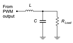
Figure \(\PageIndex{3}\): Passive low-pass filter.

At low frequencies, \(X_L\) will be very small while \(X_C\) will be very high, thus virtually all of the input signal frequencies will pass on to the load. At high frequencies, such as the harmonics of the PWM pulses, the situation is reversed: \(X_L\) is large and \(X_C\) is small, creating a large loss so that these components do not reach the load.¹ The critical frequency of the network is set to the highest input signal frequency (e.g., for high fidelity audio, slightly above 20 kHz).

We now have a complete outline for the class D amplifier, as shown in Figure \(\PageIndex{4}\).

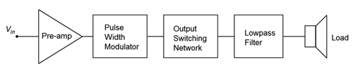
Figure \(\PageIndex{4}\): Class D amplifier block diagram.

The pre-amp can be comprised of any of the linear amplifier outlines presented in earlier chapters, whether they use BJTs or FETs. What remains then, is further investigation into the output switching network.

References

¹For an audio amplifier, it is important that these components do not reach the loudspeaker. Even though they are beyond the range of human hearing, they can damage loudspeaker sub-components and, at the very least, present an extra power dissipation burden to them. Other kinds of loads may not be effected by the harmonics and filtering may not be needed.