
3.5: Ohm's Law
- Page ID
- 25109

In Chapter 2, the concept of resistance was introduced using the following generality:
\[Effect = \frac{Cause}{Oppostion} \nonumber \]
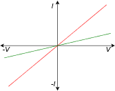
Figure 3.5.1 : Current-voltage plots for simple resistors.
To review, the cause is a voltage source, the opposition is the resistance, and the effect is the resulting current. If the item the current passes through is linear, such as the simple resistors depicted in Figure 3.5.1 , then this relationship can be rewritten as:
\[I = \frac{V}{R} \nonumber \]
or more commonly, solved for the voltage and expressed as:
\[V = I \times R \label{3.3} \]
This is called Ohm's law, and is named in honor of Georg Ohm, a researcher from the early nineteenth century. It is, along with Kirchhoff's laws that we shall see shortly, one of the most important and useful equations available for the analysis of DC electrical circuits. For the sake of completeness, Ohm's law can also be visualized in terms of resistance:
\[R = \frac{V}{I} \nonumber \]
All three forms of this equation are useful. For example, we can use the first version if we have a known voltage applied across a resistor and we want to determine the resulting current. Similarly, Equation \ref{3.3} can be used to find the voltage drop across a resistor if we know the current through it. Finally, we can use the last version if we need to set the current to a certain value and have to find the resistance required to do so.
A 9 volt battery is used in series to power a 40 \( \Omega \) resistor as shown in Figure 3.5.2 . Determine the circulating current. Also determine the minimum power rating for the resistor.
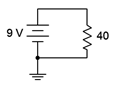
Figure 3.5.2 : Circuit for Example 3.5.1 .
\[I = \frac{V}{R} \nonumber \]
\[I = \frac{9 V}{40 \Omega} \nonumber \]
\[I = 0.225amps \nonumber \]
From power law, Equation 2.5.3,
\[P = I \times V \nonumber \]
\[P = 0.225 A \times 9 V \nonumber \]
\[P = 2.025 watts \nonumber \]
Power could also be determined using \(V^2 /R\) or \(I^2R\). Try it. You should get the same result.
Computer Simulation
To verify the results of the preceding example, the circuit is entered into a simulator, as shown in Figure 3.5.3 . Multisim™ is used here, although any quality circuit simulator will do. Virtual DMMs are used to measure the current and voltage. Remember, current is the rate of charge flow and is measured at a single point; the middle of a connecting wire if you will. Consequently, the ammeter is inserted between the battery and resistor. In contrast, voltage is a potential difference which implies two points for the measurement, and thus, the voltmeter is placed across the resistor.
Note the voltage is exactly 9 volts as expected. The current is just shy of the expected 225 milliamps. This is due to the fact that all real world ammeters exhibit some finite internal resistance. This extra resistance, though very much smaller than the resistor, adds to the total resistance and thus slightly decreases the current. The simulator has been programmed to mimic this behavior and thus we see a very slight decrease in the current in the simulation, which is precisely the effect we would see in a proper physical lab.
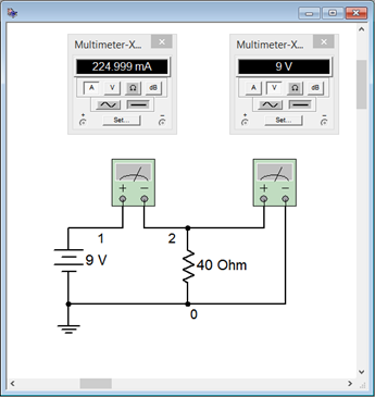
Figure 3.5.3 : The circuit of Example 3.5.1 in a simulator.
This simulation uses virtual instruments because they echo the layout of a physical lab and offer some familiarity. Unfortunately, they become cumbersome in larger circuits. We shall look at other, more direct, simulation techniques later in this chapter.
Refer to the battery and lamp circuit shown back in Figure 3.3.1. Determine the resistance of the lamp if the current flowing through it is 300 mA and the battery voltage is 6 volts. Also determine the power dissipated by the lamp.
\[R = \frac{V}{I} \nonumber \]
\[R = \frac{6 V}{0.3A} \nonumber \]
\[R = 20 \Omega \nonumber \]
From power law,
\[P = I^2 \times R \nonumber \]
\[P = 0.3A^2 \times 20 \Omega \nonumber \]
\[P = 1.8 watts \nonumber \]
Let's continue with a couple of examples utilizing current sources.
Determine the voltage developed across the resistor in the circuit of Figure 3.5.4 . Also determine the power dissipated.
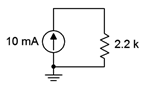
Figure 3.5.4 : Circuit for Example 3.5.3 .
\[V = I \times R \nonumber \]
\[V = 10 mA \times 2.2k \Omega \nonumber \]
\[V =22 volts \nonumber \]
From power law,
\[P = I^2 \times R \nonumber \]
\[P = (10 mA)^2 \times 2.2 k \Omega \nonumber \]
\[P = 0.22 watts \nonumber \]
Computational hint: don't forget the “milli” part of the current (milli squared is micro).
Determine the resistor value required in the circuit of Figure 3.5.5 in order for the source to generate 24 watts of power.
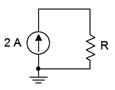
Figure 3.5.5 : Circuit for Example 3.5.4 .
First, note that power generated must equal power dissipated. Thus, the power generated by the source must equal the power dissipated by the resistor. From power law,
\[P = I^2 \times R \nonumber \]
\[R = \frac{P}{I^2} \nonumber \]
\[R = \frac{24 W}{(2 A)^2} \nonumber \]
\[R = 6 \Omega \nonumber \]
As a crosscheck, note that Ohm's law indicates that a 6 \( \Omega \) resistor would produce a 12 volt drop given a 2 amp current, and that 12 volts times 2 amps yields the expected 24 watts.
It is now time to move onto series circuits using multiple resistors and/or current sources.