
3.7: Series Analysis
- Page ID
- 31678

Ohm's law, Kirchhoff's voltage law, the voltage divider rule and series component combinations are the tools we will use to solve general series circuit problems. There are multiple techniques for analyzing these circuits:
- If all voltage source and resistor values are given, the circulating current can be found by dividing the equivalent voltage by the sum of the resistances. Once the current is found, Ohm's law can be used to find the voltage drops across individual resistors. Alternately, the individual voltage drops can be found using the voltage divider rule. At that point, power law can be used to find the power dissipation in each resistor or the power developed by the source(s).
- If the circuit uses a current source instead of a voltage source, then the circulating current is known and the voltage drop across any resistor may be determined directly using Ohm's law.
- If the problem concerns determining resistance values, the basic idea will be to use these rules in reverse. For example, if a resistor value is needed to set a specific current, the total required resistance can be determined from this current and the given voltage supply. The values of the other series resistors can then be subtracted from the total, yielding the required resistor value. Similarly, if the voltages across two resistors are known, as long as one of the resistance values is known, the other resistance can be determined using either the voltage divider rule or Ohm's law.
Often, there will be more than one way to solve a given problem. We shall refer to these as solution paths. No particular path is “more correct” than any other, although some paths may be shorter or easier in a given case, as will be illustrated next.
Determine the voltage \(V_b\) (i.e., the voltage across the 100 \(\Omega \) resistor) in the circuit of Figure 3.7.1 . Also determine the circulating current.
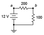
Figure 3.7.1 : Circuit for Example 3.7.1 .
First, note that there is a single voltage source that will create a clockwise current flowing through the two resistors. KVL says that the combined drops across those resistors must equal the rise of the source, or 12 volts. One solution path involves first finding the total resistance. Dividing this into the source voltage will yield the current. Ohm's law can then be used to determine the resistor voltage.
\[R_T = R_1+R_2 \nonumber \]
\[R_T = 200 \Omega +100 \Omega \nonumber \]
\[R_T = 300 \Omega \nonumber \]
\[I = \frac{E}{R_T} \nonumber \]
\[I = \frac{12 V}{300\Omega} \nonumber \]
\[I = 40 mA \nonumber \]
\[V_b = I \times R_2 \nonumber \]
\[V_b = 40 mA \times 100\Omega \nonumber \]
\[V_b = 4 \text{ volts} \nonumber \]
A second solution path involves first finding the resistor voltage via the voltage divider rule. The current can then be found via Ohm's law.
\[V_b = E \frac{R_2}{R_T} \nonumber \]
\[V_b = 12V \frac{100 \Omega}{300\Omega} \nonumber \]
\[V_b = 4 \text{ volts} \nonumber \]
\[I = \frac{V_b}{R_2} \nonumber \]
\[I = \frac{4V}{100 \Omega} \nonumber \]
\[I = 40 mA \nonumber \]
Computer Simulation
Let's verify the preceding example using a computer simulation. Instead of using virtual instruments, we shall use a more direct route, namely a listing of node voltages. A node voltage is the voltage at a given point with respect to some other point, normally ground, as in \(V_b\) in the prior example. Note that as we treat connecting wires ideally (having no resistance), a node is the entire connection wire, not a specific location on it. Normally, simulators will automatically number each node in a circuit with ground being node 0. This method skips the entire business of inserting virtual meters in the circuit and reduces schematic clutter.
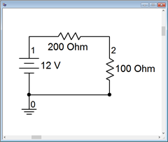
Figure 3.7.2 : The circuit of Example 3.7.1 in the simulator.
Note that ground is node 0, the power supply connection to the first resistor is node 1 and the connection between the two resistors is node 2. Thus, node 2 is \(V_b\). A DC operating point analysis is performed. The results are shown in a separate output window, as depicted in Figure 3.7.3 . The values are as expected and with no loading effects as might be seen with virtual instruments.
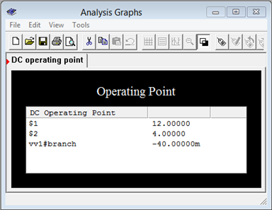
Figure 3.7.3 : Simulation results for the circuit of Figure 3.7.2 .
Determine the voltage \(V_a\) (i.e., the voltage across the current source) in the circuit of Figure 3.7.4 .
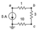
Figure 3.7.4 : Circuit for Example 3.7.2 .
Given the direction of the current source, the current will flow counterclockwise. This produces voltage drops (plus to minus) left to right across the 10 \(\Omega \), bottom to top across the 3 \(\Omega \), and right to left across the 1 \(\Omega \) resistor. This means that node \(a\) is negative with respect to ground (i.e., the voltage keeps dropping across the resistors as we travel counterclockwise from ground, indicating that the resulting potential keeps getting more and more negative with respect to ground). To find \(V_a\), we may simply sum the resistors and then use Ohm's law to determine their combined voltage drop, which of course, must equal the voltage rise from the current source.
\[R_T = R_1+R_2+R_3 \nonumber \]
\[R_T = 1\Omega +3\Omega +10\Omega \nonumber \]
\[R_T = 14\Omega \nonumber \]
\[V_a = −I \times R_T \nonumber \]
\[V_a = −5 A \times 14 \Omega \nonumber \]
\[V_a = −70 \text{ volts} \nonumber \]
One practical point when designing circuits is to appreciate the variations in current and voltage produced by component tolerances. For example, in the preceding problem, we determined that there will be 70 volts across the current source, but this assumes that the resistor values are exactly as stated. In the previous chapter we discovered that all resistor values will vary somewhat, and we grade this variation as a percent tolerance. Thus, if the true resistor values are off a bit, we would expect this to impact the associated voltages. Often, we would like to determine worst case values such as a maximum voltage or a minimum current. Sometimes these conditions occur when all resistors are at their maximum or minimum value. For example, the maximum value of source voltage in the previous problem occurs when all of the resistor values are at their maximum. This is not always the case, though. Sometimes the minima and maxima are achieved with odd combinations, such as one resistor being at maximum and another being at minimum. For instance, in the circuit used for Example 3.7.1 , \(V_b\) will be at minimum when \(R_2\) is at minimum and when \(R_1\) is at maximum. This can be verified easily using VDR.
Computer Simulation
Along with worst case, we might also like to know the sort of typical spread we get on a particular parameter using normal component variations. This can be performed in a simulator and it is usually called Monte Carlo Analysis or something similar. Basically, the simulator computes a series of simulation runs, each with component values chosen randomly within the specified tolerances of the chosen components, mimicking the effect of pulling the components out of a parts bins. To illustrate the Monte Carlo technique, the circuit of Example 3.7.2 is entered in a simulator as shown in Figure 3.7.5 .
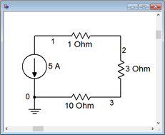
Figure 3.7.5 : The circuit of Example 3.7.2 in the simulator.
The resistors are given 10% tolerances. Five runs are specified for node voltage 1 which is equivalent to \(V_a\) in the original circuit. The results are shown in Figure 3.7.6 . Note that the nominal value run indicates −70 volts as expected. The other runs show variations on this voltage, some above and some below the nominal result.
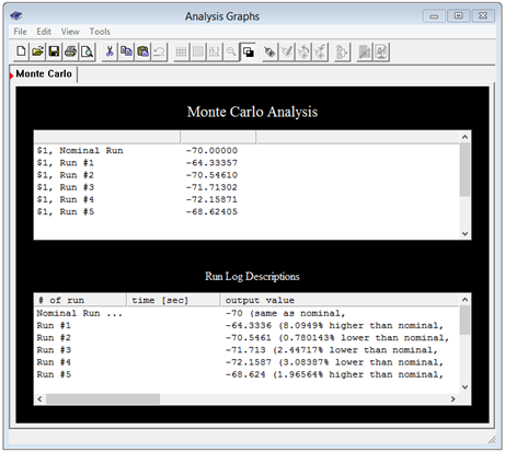
Figure 3.7.6 : Simulation results for the circuit of Figure 3.7.5 .
The Importance of Polarity
A key item of importance when analyzing series circuits, or indeed any electrical circuit, is noting the polarity of the voltages. This was apparent in Example 3.7.2 . Determining polarity for voltage sources is easy as their polarity is fixed (positive is always at the “long bar” and negative at the “short bar”). The polarity of any resistor will depend on the direction of current flow. To avoid confusion we will use the following standard:
- Where conventional current enters a resistor, we label this point with a plus sign, and where the current leaves, a minus sign.
- During analysis, moving from plus to minus is a voltage drop. That is, we are moving from a more positive or higher potential to a less positive or lower potential, thus “dropping” voltage.
- Similarly, traversing from minus to plus is a voltage rise.
Remember, Kirchhoff's voltage law states that the sum of voltage rises around a series loop must equal the sum of voltage drops.
Along with determining the voltage across single resistors, we are often interested in determining the voltage between arbitrary points in a circuit. These may span several components. It is imperative that we know the polarities of the individual voltages in order to determine the voltage between any two circuit points. The foregoing is illustrated using the series circuit schematic of Figure 3.7.7 .
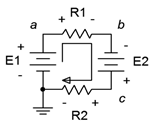
Figure 3.7.7 : A multi-source, multi-resistor series circuit.
Here, the two voltage sources, \(E_1\) and \(E_2\), aid each other because they are both trying to establish a clockwise current. This produces a net voltage of \(E_1+E_2\). Their polarities are fixed. The current direction will be as drawn because conventional current flows out of the positive terminal of a voltage source. The value of this current will be \((E_1+E_2) / (R_1+R_2)\) via Ohm's law. Knowing the direction of current, the polarities of the voltage drops across the two resistors may be found. The point where the current enters the resistor is positive, and negative where it exits. Once these are labeled, either Ohm's law or the voltage divider rule can be used to determine the voltages developed across the two resistors. Note that KVL states that the sum of these two resistor voltages must equal the net supplied voltage, or \(E_1+E_2\) in this case.
To determine the voltage from point \(a\) to point \(c\), or \(V_{ac}\), we start at point \(a\) and sum the voltage drops and rises until we get to point \(c\). Here, the voltage across \(R_1\) shows up as a drop (+ to − and taken as positive) and the voltage across \(E_2\) shows up as a rise (− to +, and thus negative). The result is the voltage across \(R_1\) minus the voltage across \(E_2\). Depending on the specific values, the sum may wind up being either a positive or negative value. If it's positive, this signifies that point \(a\) is at a higher potential than is point \(c\). Conversely, if it's negative, this signifies that point \(a\) is at a lower potential than is point \(c\). If we reverse the order, starting at point \(c\) and moving to point \(a\), or \(V_{ca}\), we will wind up with the same voltage magnitude but the sign will flip. In the laboratory, the first point letter (the \(a\) in \(V_{ac}\)) is where the red lead of the voltmeter is connected and the second letter is where the black lead is connected. As a reminder, if a single connection point is used, as in \(V_a\), the second letter is assumed to be ground. Thus, \(V_a\) is the voltage from point \(a\) to ground.
To illustrate the importance of voltage source polarity, consider the series circuit shown in Figure 3.7.8 . This circuit is identical to the previous circuit with the exception that the polarity of source \(E_2\) has been flipped. This can have a drastic change on the resulting current and voltage drops. For example, if \(E_2\) is larger than \(E_1\), the net supplied voltage will be \(E_2−E_1\) and the direction of conventional current will be as drawn. Effectively, \(E_2\) will be charging \(E_1\). Note that this is opposite to the prior circuit. Because both the direction and the magnitude of the current have changed, the voltage drops and polarities of \(R_1\) and \(R_2\) will change. Consequently, any point-to-point voltage, such as \(V_{ac}\), will also change.
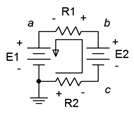
Figure 3.7.8 : Series circuit with altered polarity.
Determine the voltages \(V_b\) and \(V_{ca}\) in the circuit of Figure 3.7.9 .

Figure 3.7.9 : Circuit for Example 3.7.3 .
The first step here would be to note that the two sources are in opposition. The result is an effective source of 10.5 volts with the same polarity as the 12 volt source, meaning it creates a clockwise current (rather the opposite of Figure 3.7.8 ). The total resistance will be the sum of the resistors, or 500 \(\Omega \). From this we can compute the current and then the voltage drops across each resistor. The polarity across the 100 \(\Omega \) will be + to − left to right, and across the 400 \(\Omega \) it will be + to − right to left. The polarities for both sources are top to bottom + to −. This is shown in Figure 3.7.10 .
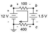
Figure 3.7.10 : Circuit for Example 3.7.3 with current direction and voltage polarities shown.
\[I = \frac{E_{Total}}{R_{Total}} \nonumber \]
\[I = \frac{10.5 V}{500 \Omega} \nonumber \]
\[I = 21 mA \nonumber \]
\[V_{100} = I \times R_{100} \nonumber \]
\[V_{100} = 21 mA \times 100\Omega \nonumber \]
\[V_{100} = 2.1 \text{ volts} \nonumber \]
\[V_{400} = I \times R_{400} \nonumber \]
\[V_{400} = 21 mA \times 400\Omega \nonumber \]
\[V_{400} = 8.4 \text{ volts} \nonumber \]
To find \(V_b\) we start at node \(b\) and work our way to ground, summing the potentials as we go. First we see the 1.5 volt source. Even though this is a source, it is still considered a voltage drop because the polarity is + to −. The polarity on the 400 \(\Omega \) resistor is the same, so we add in its 8.4 volts for 9.9 volts total. That is, node \(b\) is 9.9 volts above ground.
For \(V_{ca}\) we proceed similarly. Starting at node \(c\) we move through the 1.5 volt source, but this time the polarity is − to +, or a rise of 1.5 volts (i.e., taken as negative). Now at node \(b\), we continue through the 100 \(\Omega \) resistor, also seeing a − to + polarity, or a rise of 2.1 volts. That adds up to 3.6 volts in magnitude, however, the starting node is lower than the ending node, thus \(V_{ca}\) = −3.6 volts. We could also say \(V_{ac}\) = 3.6 volts.
Back in Chapter 2 the height analogy for voltage was presented. This can be applied nicely in the prior example. You can think of ground as literally ground: the earth under your feet. Voltage rises would be like climbing up a ladder and voltage drops would be like climbing down a ladder. Think of each volt as being analogous to one foot or one meter. Thus, for \(V_b\), you climb up the ladder 8.4 feet for the 400 \(\Omega \) and another 1.5 feet for the 1.5 volt source, leaving you 9.9 feet (volts) above the ground. Therefore, \(V_b\) must be positive with respect to ground by 9.9 volts. This analogy works for voltages below ground as well: just think in terms of digging a hole. For voltages that are not referenced to ground, think of climbing up and down ladders, and then comparing the height of where you stopped to the height of where you started.
Precisely labeling every voltage polarity may seem like unnecessary work, but as circuit complexity increases so does the opportunity for polarity errors. This important step should not be omitted. Consider the following example which is only slightly more complex than the one preceding.
Determine the voltage \(V_{be}\) in the circuit of Figure 3.7.11 .
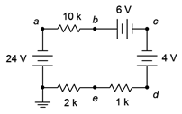
Figure 3.7.11 : Circuit for Example 3.7.4 .
The 24 volt and 6 volt sources are aiding each other while the 4 volt source is in opposition. The result is an effective supplied potential of 26 volts with a current circulating counterclockwise. The current direction and voltage polarities are shown in Figure 3.7.12 .
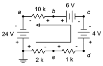
Figure 3.7.12 : Circuit for Example 3.7.4 with current direction and voltage polarities shown.
First, find the circulating current and then find the voltage drops across the resistors of interest. The total resistance is the sum of the three, or 13 k\(\Omega \).
\[I = \frac{E_{Total}}{R_{Total}} \nonumber \]
\[I = \frac{26 V}{13 k \Omega} \nonumber \]
\[I = 2 mA \nonumber \]
\[V_{10k} = I \times R_1 \nonumber \]
\[V_{10k} = 2 mA \times 10 k \Omega \nonumber \]
\[V_{10k} = 20 \text{ volts} \nonumber \]
Similarly, \(V_{2k}\) = 4 volts and \(V_{1k}\) = 2 volts with the polarities shown. To determine \(V_{be}\), we can start at node \(b\) and move to node \(e\) by either going to the left or right side. We shall do both and compare the results.
Going to the left, we see + to − 20 volts across the 10 k\(\Omega \), − to + 24 across the left side source, and then + to − 4 volts across the 2 k\(\Omega \). This adds up to 0 volts, meaning that nodes \(b\) and \(e\) are at the same potential! Double checking by going down the right side we see + to − 6 volts for the top source, − to + 4 volts for the right side source, and finally − to + 2 volts for the 1 k\(\Omega \). This is also 0 volts, as expected.
It is important to understand that saying \(V_{be}\) = 0 volts does not imply that \(V_b\) or \(V_e\) are 0 volts. In fact, we can see that \(V_e\) is below ground by the voltage dropped across the 2 k\(\Omega \), or −4 volts. Similarly, \(V_b\) is above node \(a\) by 20 volts, and node \(a\) itself is 24 volts below ground given the polarity of the left side source. The result, once again, is −4 volts.
One more example to better illustrate the voltage divider rule in a larger circuit.
Determine the voltages, \(V_b\), \(V_d\), and \(V_{bd}\) in the circuit of Figure 3.7.13 .
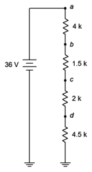
Figure 3.7.13 : Circuit for Example 3.7.5 .
While we could find the circulating current, then use Ohm's law to find the individual voltage drops, and finally add these pieces to find the potentials we're looking for, we shall instead focus on using VDR which may be faster.
The voltage divider rule states that the voltage across any resistor or group of resistors in a series loop is proportional to their resistance compared to the total resistance in that loop. The total resistance in this circuit is 12 k\(\Omega \). To find the voltage across any resistor or group of resistors, we simply make a ratio of the resistance of interest to the total resistance and multiply by the applied source voltage. Numbering the resistors R\(_1\) at top to R\(_4\) at bottom:
\[V_d = E \frac{R_4}{R_T} \nonumber \]
\[V_d = 36 V \frac{4.5 k\Omega}{12 k\Omega} \nonumber \]
\[V_d = 13.5 \text{ volts} \nonumber \]
\[V_b = E \frac{R_2+R_3+R_4}{R_T} \nonumber \]
\[V_b = 36V \frac{8k \Omega}{12 k \Omega} \nonumber \]
\[V_b = 24 \text{ volts} \nonumber \]
\[V_{bd} = E \frac{R_2+R_3}{R_T} \nonumber \]
\[V_{bd} = 36 V \frac{3.5 k \Omega}{12 k\Omega} \nonumber \]
\[V_{bd} = 10.5 \text{ volts} \nonumber \]
There is another way to find \(V_{bd}\) here, and that's to notice that by definition \(V_{bd} = V_b − V_d\). Therefore, \(V_{bd}\) = 24 volts − 13.5 volts, or 10.5 volts.