10.2: Electromagnetic Induction

Perhaps the most important observation regarding magnetic systems is Faraday's law of electromagnetic induction. Briefly, it states:

\[\text{If a conductor is cut by changing magnetic lines of force, a voltage will be induced in the conductor.} \label{10.1} \]

More specifically,

\[e = − \frac{d \Phi}{dt} \label{10.2} \]

Where

\(e\) is the induced voltage,

\(d\Phi /dt\) is the rate of change of magnetic flux with respect to time.

Therefore, the larger the flux and the more quickly it fluctuates, the greater the induced voltage. What is important here is a relative change with respect to the conductor and field. This can be accomplished in two basic ways: by a magnetic field that is itself fluctuating around a fixed conductor, or by a conductor moving through a magnetic field.

The concept of electromagnetic induction is a key element of a variety of transducers. Simply put,

\[\text{A transducer is a device that transforms energy from one type to another.} \label{10.3} \]

Although many people don't think of them as such, electric motors and generators are perfect examples of transducers. An electric motor transforms electrical energy into mechanical energy and a generator does the precise opposite, transforming mechanical energy into electrical energy. More commonly, the word transducer is associated with devices such as loudspeakers and microphones. A loudspeaker transforms its electrical input into an acoustic pressure wave (sound) whereas the microphone performs the complementary function of transforming an acoustic pressure wave into an electrical signal. While there are different ways of constructing these devices, the most common designs are the dynamic loudspeaker and dynamic microphone, both of which rely on the principle of electromagnetic induction. The designs of the two devices are strikingly similar, mostly varying in size and parts optimization. Let's take a closer look at how they operate.

Dynamic Loudspeakers and Microphones

Regardless of their output capabilities and frequency range, all dynamic loudspeakers share a common set of elements. Corresponding elements can be found in dynamic microphones. Indeed, the devices are so similar that in some applications, small loudspeakers might pull double duty and switch over to a microphone mode of operation. A cutaway view of a loudspeaker designed to reproduce low frequencies is shown in Figure 10.2.1 .

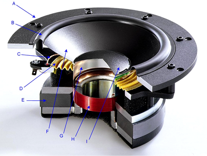
Figure 10.2.1 : Cutaway view of a dynamic loudspeaker. A. Frame B. Suspension C. Lead wire D. Spider E. Magnet F. Diaphragm G. Voice coil former H. Voice coil I. Dust cap Image courtesy of Audio Technology.

The heart of the system is a voice coil (H) which is a coil of tightly wound magnet wire. This sits inside of a magnetic field that is created by a powerful permanent magnet (E). The voice coil is connected to a diaphragm (F) that is is usually made of paper or plastic. This assembly is connected to the frame by the spider (D) at the top of the voice coil, and a suspension at the end of the diaphragm (B). The voice coil and diaphragm can move back and forth relative to the frame, like a piston.

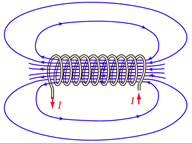
Figure 10.2.2 : Magnetic field around a coil. Image ©, courtesy of HyperPhysics

To understand the operation, recall that passing a current through a coil of wire creates a magnetic field around the coil, as illustrated in Figure 10.2.2 . This magnetic field is the same as is created by a normal magnet. In this case the north pole is on the left side (i.e., lines of force exiting). Consequently, this coil will interact with a permanent magnet just like any other magnet would. In the case of the loudspeaker, the voice coil is fed a current from the amplifier that echoes the music or voice signal. This current creates a magnetic field around the voice coil which interacts with the field of the permanent magnet. As the direction of the current changes, the poles of the voice coil's field reverse. Thus, sometimes the voice coil is pushed outward and sometimes it is pulled inward. Further, the larger the current, the greater the field it creates, and the greater the push or pull.

This results in a back-and-forth motion of the diaphragm that echoes the shape of the waveform being fed from the amplifier. As the diaphragm pushes against the air, it sets up a pressure wave, and we have sound.

A dynamic microphone runs the sequence in reverse. First, the diaphragm will move back and forth in accordance to an applied sound wave. This causes the voice coil to move back and forth within the field of the permanent magnet. We now have a coil of wire being cut by magnetic lines of force, and by Faraday's law of induction, this means that a voltage will be induced in the coil. As long as the diaphragm can respond to the subtle changes in the acoustic pressure wave, then the resulting induced voltage should be of high fidelity. Clearly, to do this with great accuracy, the diaphragm/voice coil/suspension assembly will need to very light and nimble, meaning that the components of the microphone will tend to be much smaller than those of a loudspeaker.

Electric Guitar Pickup

A set of pickups for an electric guitar is shown in Figure 10.2.3 . Although it might be tempting to think that the pickups are just microphones, they are not. If you have any doubt of this statement, just try screaming into a guitar pickup and listen to what comes out¹. The operation of the guitar pickup does, however, rely on Faraday's law.

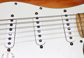
Figure 10.2.3 : Pickups on an electric guitar.

As discussed in the prior chapter covering inductance, an electric guitar pickup consists of thousands of turns of very fine wire around a permanent magnet. The pickup is placed immediately below the guitar strings. In this position, the metal guitar strings (generally various combinations of steel, nickel and/or cobalt), are within the field generated by the magnet. When a string is plucked, it vibrates in a complex pattern that depends on the note it is tuned to and the overtones that are present. This pattern distorts the magnetic field because the strings have a much higher permeability than the air around them. We now have a changing magnetic field, in the middle of which is large coil of wire. Faraday's law states that a voltage must be induced in this coil, and that it will follow the motions of the strings. This induced voltage is then fed to an amplifier, hopefully, set to 11.

The astute observer might ask, “Why are there multiple pickups?” Perhaps surprisingly, it is not to get a larger, and thus louder, signal. It has to do with the timbre, or tone quality, of the sound. When a guitar string vibrates, its motion can be thought of as containing the myriad motions of the fundamental pitch and all of the overtones that go with it. Towards the bridge, where the strings are attached, the lowest pitched elements produce little motion, and thus their strength in the overall signal is reduced. The result is that a pickup placed closer to the bridge sounds “thin” or “cutting” while one placed further up sounds “full” or “thick”.

Bicycle Computer

Our third and final illustrative example is that of a bicycle computer. These handy little devices consist of a small sensor system on the front wheel which is connected to a display unit mounted on the handlebars. Typically, these units will display current speed, average speed, elapsed time, distance covered, and other attributes of interest.

Figure 10.2.4 : Bicycle computer sensor and magnet.

The sensing apparatus of a typical bicycle computer is shown in Figure 10.2.4 . This apparatus consists of two parts: a permanent magnet mounted to one of the wheel spokes, and a weatherproof sensing unit mounted to the front fork. The principle of operation is fairly straightforward: each time the while rotates, the magnet attached to the spoke swings by the sensor. The moving magnetic field creates a short-lived voltage spike in the sensor, an example shown in Figure 10.2.5 . The computer records these spikes over time. Knowing the circumference of the wheel, a simple multiplication yields the accumulated distance traversed. Given internal clocking circuitry, the time recorded between the pulses can be turned into a velocity. Given these data, other attributes such as average or maximum speed are easily obtained with further computation.

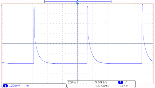
Figure 10.2.5 : Sensor signal feeding bicycle computer.

Using the oscilloscope trace shown in Figure 10.2.5 as an example, we can see that the time between the pulses is about 3.5 divisions, with each division being 200 milliseconds in length. This gives one rotation every 0.7 seconds, or roughly 5140 revolutions per hour. The sensor was mounted on a bike with 700 by 25 mm tires which yields a circumference of about 2.1 meters. Thus, the velocity would be 5140 revolutions per hour at 2.1 meters per revolution, or about 10.8 km/h (\(\approx\) 6.73 MPH).²

References

¹A little string resonance if you're lucky, and some irritated band-mates if you're not.

²In reality, the bike was mounted on a maintenance stand so its velocity was, in fact, zero. Running alongside a bike with an oscilloscope and probes is no easy feat, especially when the scope needs AC power.