
10.3: Magnetic Circuits
- Page ID
- 25023

Magnetic circuits include applications such as transformers and relays. A very simple magnetic circuit is shown in Figure 10.3.1 .
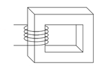
Figure 10.3.1 : Simple magnetic circuit.
First, it consists of a magnetic core. The core may be comprised of a single material such as sheet steel but can also use multiple sections and air gap(s). Around the core is at least one set of turns of wire, i.e., a coil formed around the core. Multiple sets of turns are used for transformers (in the simplest case, one for the primary and another for the secondary). As we have seen already, passing current through the windings generates a magnetic flux, \(\Phi\), in the core. As this flux is constrained within the cross sectional area of the core, \(A\), we can derive a flux density, \(B\).
\[B = \frac{\Phi}{A} \label{10.4} \]
Where
\(B\) is the magnetic flux density in teslas,
\(\Phi\) is the magnetic flux in webers,
\(A\) is the area in square meters.
Recall from Chapter 9 that one tesla is defined as one weber per square meter. An alternate unit that is sometimes used is gauss (cgs system of units), named after Carl Friedrich Gauss, the German mathematician and scientist.
\[1 \text{ tesla }= 10,000 \text{ gauss} \label{10.5} \]
A magnetic flux of 6E−5 webers exists in a core whose cross section has dimensions of 1 centimeter by 2 centimeters. Determine the flux density in teslas.
First, convert the dimensions to meters to find the area. There are 100 centimeters to the meter.
\[A = width \times height \nonumber \]
\[A = 0.01 m \times 0.02 m \nonumber \]
\[A = 2E-4 m^2 \nonumber \]
\[B = \frac{\Phi}{A} \nonumber \]
\[B = \frac{6E-5Wb}{2E-4 m^2} \nonumber \]
\[B = 0.3T \nonumber \]
Ohm's Law for Magnetic Circuits (Hopkinson's or Rowland's Law)
There is a common parallel drawn between magnetic circuits and electrical circuits, namely Hopkinson's law (Rowland's law). For electrical circuits, Ohm's law states:
\[V = I R \nonumber \]
In like manner, for magnetic circuits, we have:
\[\boldsymbol{F} = \Phi \boldsymbol{R} \label{10.6} \]
Where
\(\boldsymbol{F}\) is the magnetomotive force (or MMF) in amp-turns,
\(\Phi\) is the magnetic flux in webers,
\(\boldsymbol{R}\) is the reluctance of the material in amp-turns/weber.
The magnetomotive force compares to a source voltage or electromotive force (EMF), the magnetic flux is likened to the flow of current, and the reluctance stands in for resistance (i.e., on the one hand we have a material that resists the flow of current, and on the other, a material in which there is “reluctance” to establish magnetic flux). Further, magnetomotive force is the product of the current flowing through a coil and the number of loops or turns in the coil:
\[\boldsymbol{F} = N I \label{10.7} \]
Where
\(\boldsymbol{F}\) is the magneto-motive force in amp-turns,
\(N\) is the number of loops or turns in the coil,
\(I\) is the current in the coil in amps.
The equation for reluctance has a nice parallel with the equation for resistance (Equation 2.11 from Chapter 2):
\[R = \frac{\phi l}{A} \nonumber \]
\[\boldsymbol{R} = \frac{l}{\mu A} \label{10.8} \]
Where
\(\boldsymbol{R}\) is the reluctance in amp-turns/weber,
\(l\) is the length of the material in meters,
\(A\) is the cross sectional area of the material in square meters,
\(\mu\) is the permeability of the material in henries/meter.
Given the characteristics of the coil and the path length of the magnetic circuit, the magnetic flux gives rise to a magnetizing force, \(H\).
\[H = \frac{N I}{l} \label{10.9} \]
Where
\(H\) is the magnetizing force in amp-turns/meter,
\(N\) is the number of turns or loops in the coil,
\(I\) is the coil current in amps,
\(l\) is the length of the magnetic path in meters.
Equation \ref{10.8} reveals that ferromagnetic materials (i.e., materials that have high permeability, such as steel) produce a low reluctance. The practical problem here is that \(\mu\), unlike the resistivity \(\rho\) of resistors, is not a constant for these sorts of materials. It can vary considerably, as seen in the general diagram presented in Figure 10.3.2 . As a result, it is impractical to find reluctance in same manner that we find resistance. All is not lost, though.
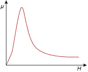
Figure 10.3.2 : Typical permeability curve for a high permeability material.
The flux density and corresponding magnetizing force for any given material are related by the following equation:
\[B = \mu H \label{10.10} \]
Where
\(B\) is the flux density in teslas,
\(\mu\) is the permeability of the material in henries/meter,
\(H\) is the magnetizing force in amp-turns/meter.
Once again, the tricky bit here is the permeability of the core material. For air, we can use the permeability of free space, \(\mu_0\).
\[\mu_0 = 4\pi \times 10^{-7} H/m \approx 1.257 \times 10^{-6} H/m \label{10.11} \]
For other materials, such as sheet steel or cast steel, we shall take another path; namely an empirically derived curve that plots flux density \(B\) against magnetizing force \(H\). Such graphs generically are referred to as “\(BH\) curves”. An example is shown in Figure 10.3.3 . Clearly, this curve is not a nice straight line, or even an obvious, predictable function. The immediately apparent attributes are the initial steep rise which is followed by a flattening of the curve. This flattening corresponds to saturation of the magnetic material. In contrast, a plot for air would reveal a straight line with a very shallow slope. As we shall see, being able to achieve a high flux density for a given magnetizing force will result in an effective and efficient magnetic circuit. So while air has the positive attribute of not saturating, the resulting flux density is low, usually leading to lower performance.
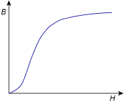
Figure 10.3.3 : Generic \(BH\) curve.
The BH Curve
The process of generating a \(BH\) curve is as follows. First, we create a core of the material to be investigated. A coil of wire is then wrapped around this core. An example is shown in Figure 10.3.4 . Here we have a basic toroid with a coil of \(N\) turns.
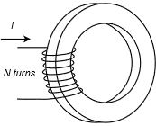
Figure 10.3.4 : Toroidal core with coil.
We begin with the system at rest and not energized. A small current, \(I\), is applied to the coil. This produces a magnetizing force via Equation \ref{10.9}. There will be a corresponding flux density, as per Equation \ref{10.10}.
The current is then increased. This produces an increase in magnetizing force and a corresponding change in flux density. The current is increased further, until the curve flattens, indicating that saturation has been reached. This trajectory is shown as the dashed line in Figure 10.3.5 , starting at point \(\boldsymbol{a}\) with point \(\boldsymbol{b}\) indicating saturation. The current is then reduced. This causes a reduction in magnetizing force, but while the flux density decreases, it does not trace back perfectly along the original trajectory. Instead, the curve is displaced above the original.
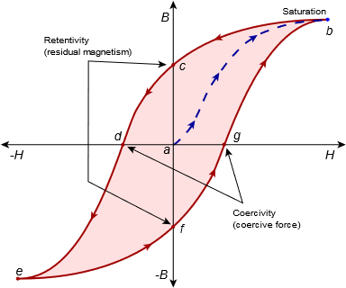
Figure 10.3.5 : Generation of BH curve.
Eventually, the current will be reduced to zero. This corresponds to point \(\boldsymbol{c}\) on the graph of Figure 10.3.5 . At this point, even though there is no current in the coil, there is still flux in the core. The resulting flux density is referred to as retentivity and is a measure of residual magnetism. This phenomenon is what makes it possible to magnetize materials.
If we now reverse the direction of the coil current and begin to increase its magnitude, the flux density will continue to drop. At point \(\boldsymbol{d}\), it will have reached zero. As we have effectively coerced the flux back to zero, we call the magnetizing force required to do this the coercivity or coercive force.
As the current magnitude increases, the flux density also increases but with opposite sign. Eventually, saturation is reached again at point \(\boldsymbol{e}\). Once again, if the current's magnitude is decreased, the magnitude of the flux density will also decrease but will not perfectly trace back along the original trajectory. This time it will follow a lower path. When the current is reduced to zero at point \(\boldsymbol{f}\), a mirror retentivity is evident. Further positive increases in current show a mirror coercivity at point \(\boldsymbol{g}\). Finally, as current is increased to maximum, we again reach saturation at point \(\boldsymbol{b}\).
If the current is cycled in this manner again, the process is repeated, and the outer path indicated by the arrows is taken again. Thus, a specific value of magnetizing force can give rise to different values of flux density: it depends on the recent history of the material. This effect is known as hysteresis and is found in other areas as well.
Effectively, published \(BH\) curves follow the middle of the hysteresis loop. An example of \(BH\) curves for three different core materials is shown in Figure 10.3.6 1. Curve A is for sheet steel (which is common in transformers), curve B is for cast steel, and curve C is for cast iron. We shall make use of these in upcoming examples. Curves for other materials are also available.
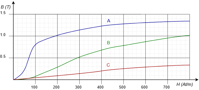
Figure 10.3.6 : BH curves for: A. Sheet steel B. Cast steel C. Cast iron
Assume the toroid of Figure 10.3.4 is made of cast steel, has a 500 turn coil, a cross section of 2 cm by 2 cm, and an average path length of 50 cm. Determine the flux in webers if a current of 0.3 amps feeds the coil.
We shall use Equation \ref{10.9} to find the magnetizing force and from the \(BH\) curve, find the flux density.
\[H = \frac{N I}{l} \nonumber \]
\[H = \frac{500 \text{ turns } \times 0.3 A}{0.5 m} \nonumber \]
\[H = 300At/m \text{ (amp-turns per meter)} \nonumber \]
Cast steel corresponds to curve B (green) in Figure 10.3.5 . A decent estimate for the flux density is 0.52 teslas. This is the corresponding flux density. In order to find the flux, we need to find the area of the core.
\[A = width \times height \nonumber \]
\[A = 0.02 m \times 0.02 m \nonumber \]
\[A = 4E-4m^2 \nonumber \]
\[\Phi = B \times A \nonumber \]
\[\Phi = 0.52 T \times 4E-4 m^2 \nonumber \]
\[\Phi = 2.08E-4Wb \nonumber \]
KVL for Magnetic Circuits
A cursory examination of Equations \ref{10.7} and \ref{10.9} shows that:
\[\boldsymbol{F} = H l = N I \label{10.12} \]
Continuing the Ohm's law analogy, the amp-turns product of the coil, \(NI\), is analogous to a voltage rise. Further, the \(Hl\) product is analogous to a voltage drop. If we then extend the analogy to include the concept of Kirchhoff's voltage law, it should come as no surprise that the sum of \(NI\) “rises” must equal the sum of the \(Hl\) “drops”. In the circuit of Figure 10.3.4 , there is a single “rise” and a single “drop”. Thus, the magnetic circuit is analogous to the minimal electric circuit shown in Figure 10.3.7 . \(\boldsymbol{F}\) is the magnetomotive force, \(NI\), while \(\boldsymbol{R}\) is the reluctance of the toroidal core. This reluctance will experience a “drop” of \(Hl\).
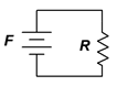
Figure 10.3.7 : Electrical circuit analogy for the magnetic system of Figure 10.3.4 .
The core could consist of two or more different materials, creating the equivalent of a series circuit. In this case, a table such as the one found in Figure 10.3.8 can be used to aid in computation. In this table, each section of the core gets its own row. The table is divided into two sides (note the thick separating line in the center). In general, we will be working through problems where we know the data on the left side and need to find something on the right side, or vice versa. The bridge between the two sides (i.e., traversing the thick line) is a \(BH\) curve for the material of that particular section. The exception to this rule is if the section is an air gap. In that case we can use Definition \ref{10.11} which shows that for air, \(H \approx 7.958E5 B\) or alternately, \(B \approx 1.257E−6 H\).
| Section |
Flux \(\Phi\) (Wb) |
Area \(A\) (m\(^2\)) |
Flux Density B (T) |
Magnetizing Force \(H\) (At/m) |
Length \(l\) (m) |
“Drop” \(Hl\) (At) |
|---|---|---|---|---|---|---|
| 1 | ||||||
| 2 |
Time for a few illustrative examples. We shall consider a simple system like that of Figure 10.3.4 , a two section core, a core with an air gap, and a core with two coils.
Assume the core of Figure 10.3.9 is made of sheet steel, has a 200 turn coil, a cross section of 1 cm by 1 cm, and an average path length of 12 cm. Determine the coil current required to achieve a flux of 1E−4 webers.
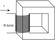
Figure 10.3.9 : Magnetic system for Example 10.3.3 .
The analogous circuit consists of a single source and reluctance, like that of Figure 10.3.7 . Thus,
\[N I = H_{sheet} l_{sheet} \nonumber \]
We shall begin by filling in the portions of the table that can be addressed directly, such as the path length, area and flux. Don't forget to convert the centimeter values into meters.
| Section |
Flux \(\Phi\) (Wb) |
Area \(A\) (m\(^2\)) |
Flux Density B (T) |
Magnetizing Force \(H\) (At/m) |
Length \(l\) (m) |
“Drop” \(Hl\) (At) |
|---|---|---|---|---|---|---|
| Sheet Steel | 1E−4 | 1E−4 | 0.12 |
Now we determine the flux density to complete the left side of the table.
\[B = \frac{\Phi}{A} \nonumber \]
\[B = \frac{1E-4 Wb}{1E-4 m^2} \nonumber \]
\[B = 1T \nonumber \]
| Section |
Flux \(\Phi\) (Wb) |
Area \(A\) (m\(^2\)) |
Flux Density B (T) |
Magnetizing Force \(H\) (At/m) |
Length \(l\) (m) |
“Drop” \(Hl\) (At) |
|---|---|---|---|---|---|---|
| Sheet Steel | 1E−4 | 1E−4 | 1 | 0.12 |
We use the \(BH\) curve of Figure 10.3.6 to find H from this flux density. From the blue curve (A) the value is about 190 amp-turns per meter.
| Section |
Flux \(\Phi\) (Wb) |
Area \(A\) (m\(^2\)) |
Flux Density B (T) |
Magnetizing Force \(H\) (At/m) |
Length \(l\) (m) |
“Drop” \(Hl\) (At) |
|---|---|---|---|---|---|---|
| Sheet Steel | 1E−4 | 1E−4 | 1 | 190 | 0.12 |
At this point we find the \(Hl\) “drop” with a simple multiplication.
| Section |
Flux \(\Phi\) (Wb) |
Area \(A\) (m\(^2\)) |
Flux Density B (T) |
Magnetizing Force \(H\) (At/m) |
Length \(l\) (m) |
“Drop” \(Hl\) (At) |
|---|---|---|---|---|---|---|
| Sheet Steel | 1E−4 | 1E−4 | 1 | 190 | 0.12 | 22.8 |
This “drop” is 22.8 amp-turns and the coil has 200 turns. Therefore the required current is:
\[I = \frac{H l}{N} \nonumber \]
\[I = \frac{22.8At}{200 t} \nonumber \]
\[I = 114mA \nonumber \]
Next, let's consider a core with two sections.
Given the magnetic system shown in Figure 10.3.10 , assume section A is made of sheet steel and section B is made of cast steel. Each part has a cross section of 2 cm by 2 cm. The path length of A is 12 cm and the path length of B is 4 cm. If the coil has 50 turns, determine the coil current required to achieve a flux of 2E−4 webers.
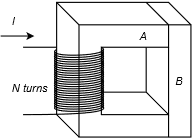
Figure 10.3.10 : Magnetic system for Example 10.3.4 .
The analogous circuit consists of a single source and two reluctances. This is shown in Figure 10.3.11 .
Therefore:
\[N I = H_{sheet} l_{sheet}+H_{cast} l_{cast} \nonumber \]
For our table there will be two rows, one for sheet steel and the second for cast steel. The first row will require using curve A (sheet steel) from Figure 10.3.6 while the second row will require using curve B (cast steel).
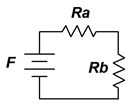
Figure 10.3.11 : Analogous electrical circuit for the system of Figure 10.3.10 .
The flux, like the current in a series loop, will be the same in both sections. From here we can fill out a series of other values in the table to arrive at:
| Section |
Flux \(\Phi\) (Wb) |
Area \(A\) (m\(^2\)) |
Flux Density B (T) |
Magnetizing Force \(H\) (At/m) |
Length \(l\) (m) |
“Drop” \(Hl\) (At) |
|---|---|---|---|---|---|---|
| Sheet Steel | 2E−4 | 4E−4 | 0.5 | 0.12 | ||
| Cast Steel | 2E−4 | 4E−4 | 0.5 | 0.04 |
The \(BH\) curves are used to transition to the right side, and we arrive at:
| Section |
Flux \(\Phi\) (Wb) |
Area \(A\) (m\(^2\)) |
Flux Density B (T) |
Magnetizing Force \(H\) (At/m) |
Length \(l\) (m) |
“Drop” \(Hl\) (At) |
|---|---|---|---|---|---|---|
| Sheet Steel | 2E−4 | 4E−4 | 0.5 | 70 | 0.12 | |
| Cast Steel | 2E−4 | 4E−4 | 0.5 | 290 | 0.04 |
And now we fill in the \(Hl\) “drops”:
| Section |
Flux \(\Phi\) (Wb) |
Area \(A\) (m\(^2\)) |
Flux Density B (T) |
Magnetizing Force \(H\) (At/m) |
Length \(l\) (m) |
“Drop” \(Hl\) (At) |
|---|---|---|---|---|---|---|
| Sheet Steel | 2E−4 | 4E−4 | 0.5 | 70 | 0.12 | 8.4 |
| Cast Steel | 2E−4 | 4E−4 | 0.5 | 290 | 0.04 | 11.6 |
Using our KVL analogy, the total “drop” is 8.4 At + 11.6 At, or 20 ampturns. The coil was specified as having 50 turns. Therefore:
\[I = \frac{H l}{N} \nonumber \]
\[I = \frac{20 At}{50 t} \nonumber \]
\[I = 400mA \nonumber \]
Notice that even though the cast steel section is shorter than the sheet steel section, it produces a larger “drop”; just like a larger resistor in an electrical circuit. This requires a larger current in the coil than if the entire core had been made of sheet steel.
Finally, it should be apparent that the current demand can be reduced if the coil has more turns. There is a practical limit here because all of the turns have to fit within the opening of the core. Once that space is full, the only way to increase the number of turns is to use finer gauge wire but doing so increases wire resistance and power loss, and also lowers maximum current capacity.
Dealing With Air Gaps
Some systems include an air gap in the core. If there is only a single material for the remainder, this will create a system like that depicted in Figure 10.3.12 . The main observation here is that the permeability of air is far below that of ferromagnetic materials and thus the gap will exhibit a relatively large reluctance compared to its path length. The obvious question then is, why would we use a gap? One possibility is an electro-magnetic relay, the internals of which are illustrated in Figure 10.3.13 .
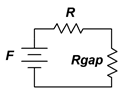
Figure 10.3.12 : Analogous electrical circuit for a system with an air gap.
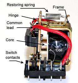
Figure 10.3.13 : Internals of an electrical relay.
To create a relay, we place one portion of the core on a hinge which can be held open with a small spring. This creates the air gap (to the immediate left of the core in the Figure). If we apply a sufficiently large current, the resulting magnetic flux will be enough to overcome the spring tension and close the second piece onto the first (i.e., magnetic attraction). Once this happens, the gap disappears, reducing the reluctance around the loop. The system will stay closed until the coil current is turned off and the restoring spring pulls apart the two sections again. We add insulated metal contacts to the moving section and what we end up with is a heavy duty switch that is “thrown” by a controlling current rather than a mechanical lever moved by a human.
It is worth repeating that for air gaps, instead of a \(BH\) curve we can use Definition \ref{10.11} which shows that for air, \(H \approx 7.958E5 B\) or alternately, \(B \approx 1.257E−6 H\).
Given the magnetic system shown in Figure 10.3.14 , assume the core is made of sheet steel. The cross section throughout is 3E−4 m\(^2\). The path length of the main core is 8 cm and the path length of the gap is 1 mm. How many turns will the coil need in order for a coil current of 400 mA to achieve a flux of 1.2E−4 webers?
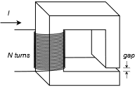
Figure 10.3.14 : Magnetic system for Example 10.3.5 .
The analogous circuit consists of a single source and two reluctances, one for the sheet steel core and a second for the air gap. This is shown in Figure 10.3.12 . Further, the analogous KVL relation is:
\[N I = H_{sheet} l_{sheet} +H_{gap} l_{gap} \nonumber \]
For this table there will be two rows, one for the sheet steel core and one for the air gap. As we have seen, the flux will be the same in both sections. From there we can fill out some of the other values in the table resulting in:
| Section |
Flux \(\Phi\) (Wb) |
Area \(A\) (m\(^2\)) |
Flux Density B (T) |
Magnetizing Force \(H\) (At/m) |
Length \(l\) (m) |
“Drop” \(Hl\) (At) |
|---|---|---|---|---|---|---|
| Sheet Steel | 1.2E−4 | 3E−4 | 0.4 | 63 | 8E−2 | |
| Gap | 1.2E−4 | 3E−4 | 0.4 | 3.183E5 | 1E−3 |
The \(BH\) curve for sheet steel and Definition \ref{10.11} for the air gap are used to transition to the right side, yielding:
| Section |
Flux \(\Phi\) (Wb) |
Area \(A\) (m\(^2\)) |
Flux Density B (T) |
Magnetizing Force \(H\) (At/m) |
Length \(l\) (m) |
“Drop” \(Hl\) (At) |
|---|---|---|---|---|---|---|
| Sheet Steel | 1.2E−4 | 3E−4 | 0.4 | 62 | 8E−2 | 5.0 |
| Gap | 1.2E−4 | 3E−4 | 0.4 | 3.183E5 | 1E−3 | 318.3 |
The \(Hl\) “drops” are filled in:
| Section |
Flux \(\Phi\) (Wb) |
Area \(A\) (m\(^2\)) |
Flux Density B (T) |
Magnetizing Force \(H\) (At/m) |
Length \(l\) (m) |
“Drop” \(Hl\) (At) |
|---|---|---|---|---|---|---|
| Sheet Steel | 1.2E−4 | 3E−4 | 0.4 | 8E−2 | ||
| Gap | 1.2E−4 | 3E−4 | 0.4 | 1E−3 |
Using our KVL analogy, the total “drop” is 5.0 At + 318.3 At, or 523.3 ampturns. The coil current was specified as being 400 mA. Therefore:
\[N = \frac{H l}{I} \nonumber \]
\[N = \frac{523.3At}{ 400mA } \nonumber \]
\[N \approx 1308 \text{ turns} \nonumber \]
And finally, an example using two coils.
Given the magnetic system shown in Figure 10.3.15 , assume the core is made of sheet steel. The cross section throughout is 3E−4 m\(^2\) and the length of the core is 20 cm. Coil one consists of 2000 turns and coil two consists of 500 turns. If a current of 120 mA into coil one achieves a flux of 2.4E−4 webers, determine the current of coil 2.
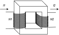
Figure 10.3.15 : Magnetic system for Example 10.3.6 .
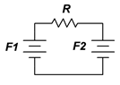
Figure 10.3.16 : Analogous electrical circuit for the system of Figure 10.3.15 .
The analogous circuit consists of two voltage sources and a single reluctance for the sheet steel core. This is illustrated in Figure 10.3.16 .
The analogous KVL relation is:
\[N_1 I_1 −N_2 I_2 = H_{sheet} l_{sheet} \nonumber \]
As we are seeking \(I_2\), we can rearrange this equation into a more useful form:
\[N_2 I_2 = N_1 I_1 −H_{sheet} l_{sheet} \nonumber \]
Only one row will be required for this table. We fill out the obvious values in the table resulting in:
| Section |
Flux \(\Phi\) (Wb) |
Area \(A\) (m\(^2\)) |
Flux Density B (T) |
Magnetizing Force \(H\) (At/m) |
Length \(l\) (m) |
“Drop” \(Hl\) (At) |
|---|---|---|---|---|---|---|
| Sheet Steel | 2.4E−4 | 3E−4 | 0.8 | 0.2 |
The \(BH\) curve for sheet steel is used to transition to the right side:
| Section |
Flux \(\Phi\) (Wb) |
Area \(A\) (m\(^2\)) |
Flux Density B (T) |
Magnetizing Force \(H\) (At/m) |
Length \(l\) (m) |
“Drop” \(Hl\) (At) |
|---|---|---|---|---|---|---|
| Sheet Steel | 2.4E−4 | 3E−4 | 0.8 | 100 | 0.2 |
The \(Hl\) “drop” is computed:
| Section |
Flux \(\Phi\) (Wb) |
Area \(A\) (m\(^2\)) |
Flux Density B (T) |
Magnetizing Force \(H\) (At/m) |
Length \(l\) (m) |
“Drop” \(Hl\) (At) |
|---|---|---|---|---|---|---|
| Sheet Steel | 2.4E−4 | 3E−4 | 0.8 | 100 | 0.2 | 20 |
Using our KVL analogy, we find:
\[N_2 I_2 = N_1 I_1 −H_{sheet} l_{sheet} \nonumber \]
\[N_2 I_2 = 2000 \text{ turns } \times 120mA −20 At \nonumber \]
\[N_2 I_2 = 240At −20 At \nonumber \]
\[N_2 I_2 = 220At \nonumber \]
Coil two was specified as having having 500 turns, therefore its current is:
\[I_2 = \frac{220 At}{500 turns} \nonumber \]
\[I_2 = 440mA \nonumber \]
An item of key importance is that the preceding example must make use of an AC current in order to function as described. A DC current will not produce the predicted results. The reason for this goes back to Definition 10.2.1 and Equation 10.2.2: Unless the flux is changing relative to the conducting coil, no voltage will be induced in a coil. So, while a DC input current will create a flux in the core, that flux will be static and unchanging. Consequently, the second coil will not produce an output. In contrast, an AC current smoothly varies in amplitude and polarity. This creates a smoothly varying magnetic flux which in turn allows a voltage to be induced in the second coil.
Assuming for a moment that an AC current was used in the preceding example, notice that the current is nearly four times higher in coil two than in coil one. If we had been able to reduce the core “drop” to zero, perhaps by reducing the core's reluctance to a negligible value, then the current would have been increased precisely by a factor four (to 480 mA versus 440 mA). This is the same as the ratio of the number of turns of coil one to the number of turns of coil two, and is known as the turns ratio. It is a key parameter describing transformers, which just happens to be the subject of the next section.
References
1Curves based on https://en.Wikipedia.org/wiki/Saturation_(magnetic); Steinmetz (1917), Theory and Calculation of Electric Circuits; and Boylestad (2010), Introductory Circuit Analysis.