1.2: Comparisons of Computer Architectures

Last updated
Save as PDF

Page ID: 27162

$ \newcommand{\vecs}[1]{\overset { \scriptstyle \rightharpoonup} {\mathbf{#1}} } $ $ \newcommand{\vecd}[1]{\overset{-\!-\!\rightharpoonup}{\vphantom{a}\smash {#1}}} $$\newcommand{\id}{\mathrm{id}}$ $ \newcommand{\Span}{\mathrm{span}}$ $ \newcommand{\kernel}{\mathrm{null}\,}$ $ \newcommand{\range}{\mathrm{range}\,}$ $ \newcommand{\RealPart}{\mathrm{Re}}$ $ \newcommand{\ImaginaryPart}{\mathrm{Im}}$ $ \newcommand{\Argument}{\mathrm{Arg}}$ $ \newcommand{\norm}[1]{\| #1 \|}$ $ \newcommand{\inner}[2]{\langle #1, #2 \rangle}$ $ \newcommand{\Span}{\mathrm{span}}$ $\newcommand{\id}{\mathrm{id}}$ $ \newcommand{\Span}{\mathrm{span}}$ $ \newcommand{\kernel}{\mathrm{null}\,}$ $ \newcommand{\range}{\mathrm{range}\,}$ $ \newcommand{\RealPart}{\mathrm{Re}}$ $ \newcommand{\ImaginaryPart}{\mathrm{Im}}$ $ \newcommand{\Argument}{\mathrm{Arg}}$ $ \newcommand{\norm}[1]{\| #1 \|}$ $ \newcommand{\inner}[2]{\langle #1, #2 \rangle}$ $ \newcommand{\Span}{\mathrm{span}}$$\newcommand{\AA}{\unicode[.8,0]{x212B}}$

This monograph is the first in a series of monographs that will cover different types of CPUs, where the two big differences between the CPU types is the address format of the instructions, and how the instruction and data memory for the processor is divided. This next section will deal with the address format of the instructions. The section following it will cover designs where instruction and data memory are combined (Von Neumann architecture) verses separate instruction and data memory (Harvard architecture).

1.2.1 Zero-, One-, and Two/Three- Address Architecture

The major difference between 0-, 1-, and 2/3- address computer architectures is where the operands for the ALU come from. This section will outline each of these architectures.

Note that in all of these architectures, operands can come from registers/memory, or operands can be part of the instruction itself. For example, the value used in the instruction add A in a one-address computer comes from memory cell at an address corresponding to the label A, and the instruction adds the value in memory location A to the $ac. In the instruction addi 5 the value of the operand is included in the instruction, and is referred to as an immediate value. In this series of monographs operators that use an immediate value will be appended with an “i”. For example, as shown above, the add instruction uses a memory value, and the addi uses an immediate value.

1.2.1.1 0-Address Architecture

When discussing the address architecture of a computer, the central question is how are the arguments to the ALU retrieved, and where are the results from the ALU stored? A 0-adress architecture retrieves (pops) the two arguments from the top of an operand stack, performs the operation, and then stores (pushes) the result back on the operand stack. The two operands to the ALU are implied as the two operands on the top of the stack, and the operation, in this case add, does not specify any operands. Because the operator does not take any explicit operands, 0 addresses are included as part of the operation and this is called a 0-address architecture. Note that a 0-address architecture is often referred to as a stack architecture because it uses a stack for the operands to/from the ALU.

Screen Shot 2020-07-02 at 6.32.49 PM.png

When writing assembly code to for this architecture, the operands are first pushed onto the stack (from memory or immediate values) using two push operations. The operation is executed, which consists of popping the two operands off the stack, running the ALU, and pushing the result back to the stack. The answer is then stored to memory by using a pop operation. The following program, which adds the value of variable A and value 5, then stores the result back to variable B, illustrates a simple 0-address program.

Program 1-1: 0-address program to add two numbers

 PUSH A
 PUSHI 5
 ADD
 POP B

Historically there have been computers implemented using 0-address architectures, such as the Burroughs 6500 and 7500 series, but it is seldom if ever used in modern hardware architectures.

However, most modern languages running on Virtual Machines (VM), such as the Java Virtual Machine (JVM) or the .Net Common Language Runtime (CLR), implement 0-address, or stack, architectures.

1.2.2 One-Address Architecture

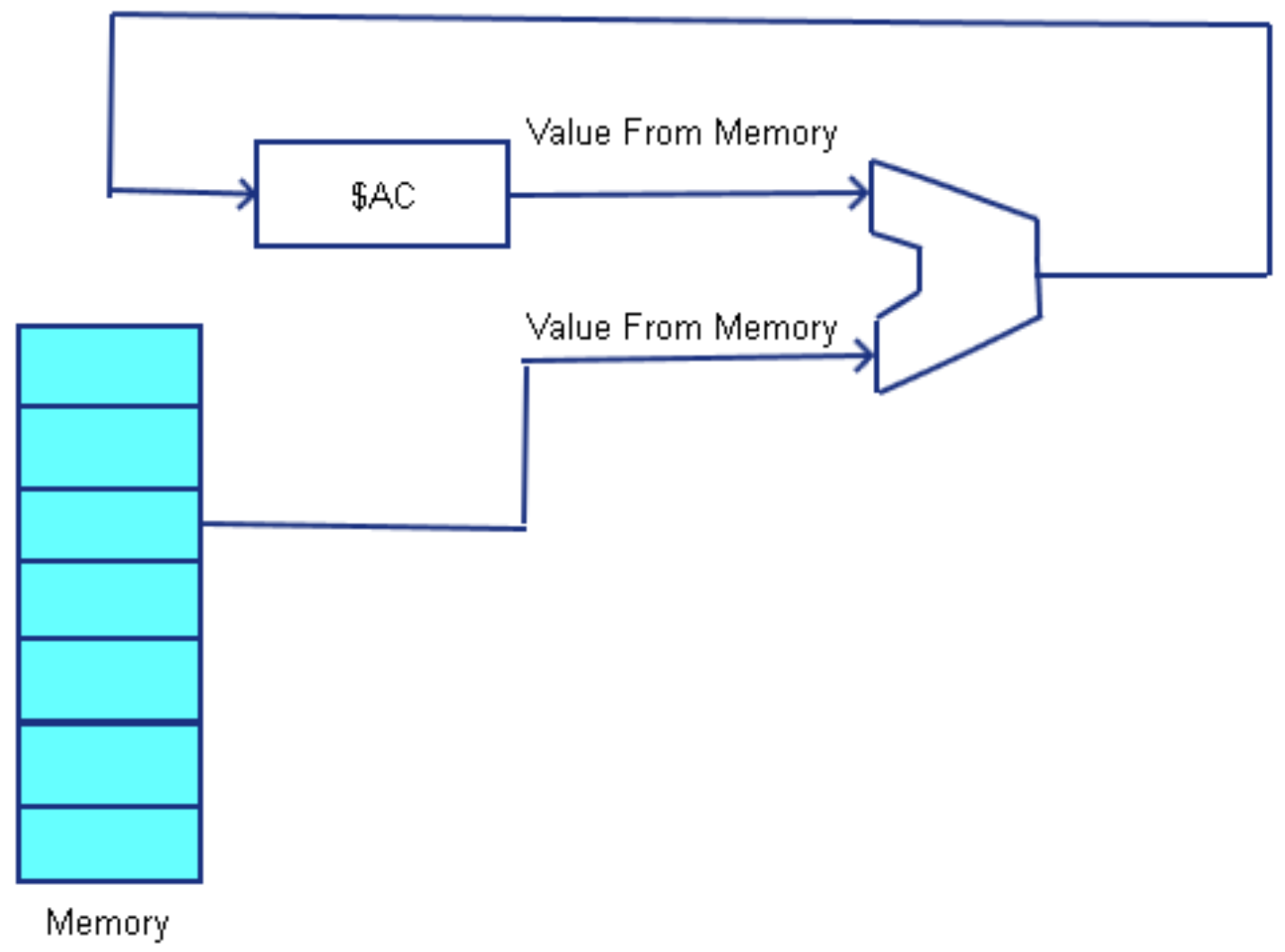
In a one-address architecture a special register, called an Accumulator or $ac is maintained in the CPU. The $ac is always an implied input operand to the ALU, and is also the implied destination of the result of the ALU operation. The second input operand is the value of a memory variable or an immediate value. This is shown in the following diagram.

Screen Shot 2020-07-02 at 6.35.48 PM.png

The following is a simple one-address computer program to add the value 5 and the value of variable A, and store the result back into variable B.

Program 1-3: one-address program to add two numbers

CLR //SettheACto0
ADDI 5 // Add 5 to the $AC. Since it was previously 0, this loads 5
ADD A // Add A+5, and store the result in the $AC
STOR B // Store the value in the $AC to the memory variable B

Because only one value is specified in the ALU operator instruction, this type of architecture is called a one-address architecture. Because a one-address architecture always has an accumulator, it is also called an accumulator architecture.

Historically many early CPUs used one-address designs, including the Intel 8080 and PDP-8, used accumulator architectures. Because of their simplicity and can be faster than other architectures, some micro-computer designs still use an accumulator architecture, though most computers implement general purpose register designs.

1.2.3 Two/Three - Address Architecture

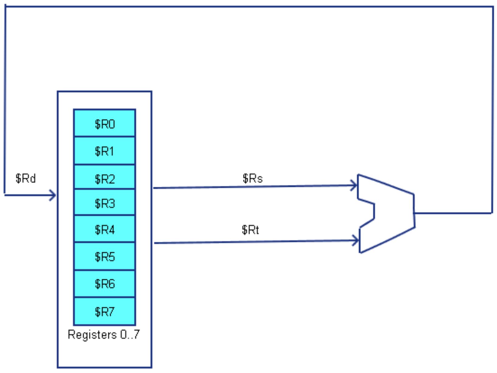
The two-address and three-address architectures are called general purpose register architectures. The two-address and three-address designs both operate in a similar fashion. Both architectures have some number of general purpose registers can be used to select the two inputs to the ALU, and the result of the ALU operation is written back to a general purpose registers. The difference is in how the result of the ALU operation (the destination register) is specified. In a three-address architecture the 3 registers are the destination (where to write the results from the ALU), R_d, and the two source registers providing the values to the ALU, R_s and R_t. This is shown in the following figure.

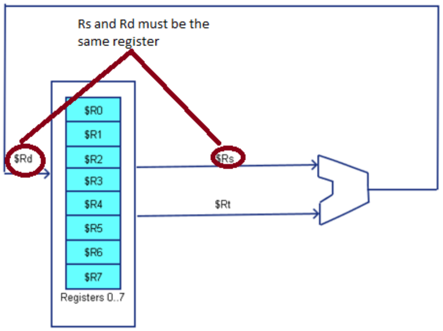
Screen Shot 2020-07-02 at 6.38.58 PM.png

A 2-address architecture is similar to a 3-address architecture, and the only difference being that only 2 registers are specified in the instruction, the first being used for both the destination of the operation and the first source to the ALU.

Screen Shot 2020-07-02 at 6.42.00 PM.png

As shown in the diagrams, the CPU selects two of the general purpose registers the values to send to the ALU, and another selection is made to write the value from the ALU back to a register. In this design, all values passed to the ALU must come from a general purpose register, and the results of the ALU must be stored in a general purpose register. This requires that memory be accessed via load and store operations, and the correct name for a two/three-address computer is a “two/three-address load/store computer”.

The following two programs execute the same program, B=A+5, as in the previous examples. The first example uses the 3-address format, and the second uses the 2-address format.

Program 1-4: 3-address program for adding two numbers

LOAD  $R0, A
LOADI $R1, 5
ADD   $R0, $R0, $R1
STORE B,   $R0

 Program 1-5: 2-address program for adding two numbers
 
LOAD  $R0, A
LOADI $R1, 5
ADD   $R0, $R1
STORE B,   $R0