The following directions detail how to use the one-address CPU.
First download the One-AddressCPU.zip file from the author’s web site, http://chuckkann.com. Unzip the file in a suitable location.
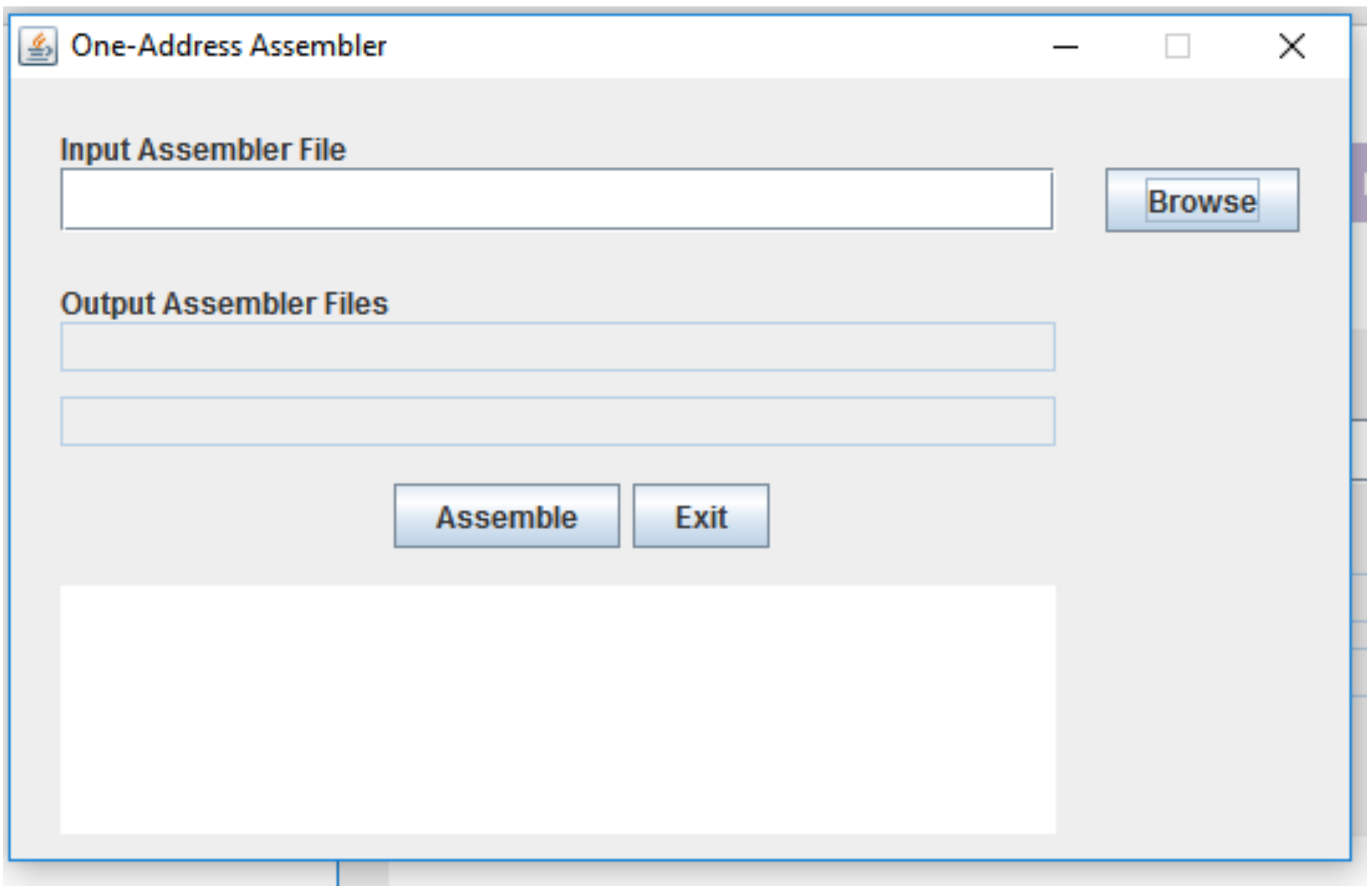
In the root directory of this zip is an executable JAR file named OneAddressAssembler.jar. Double click on this icon, and you should see the following screen.
Figure 4-3: Running the assembler - step 1
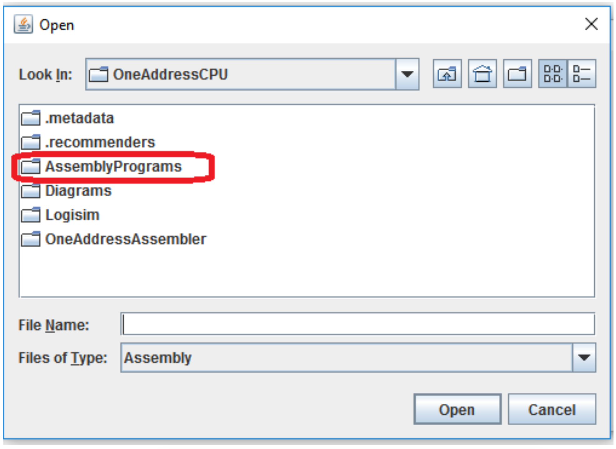
Click the Browse button, and a file dialog box should appear. Select the directory AssemblyPrograms.
Figure 4-4: Running the assembler - step 2
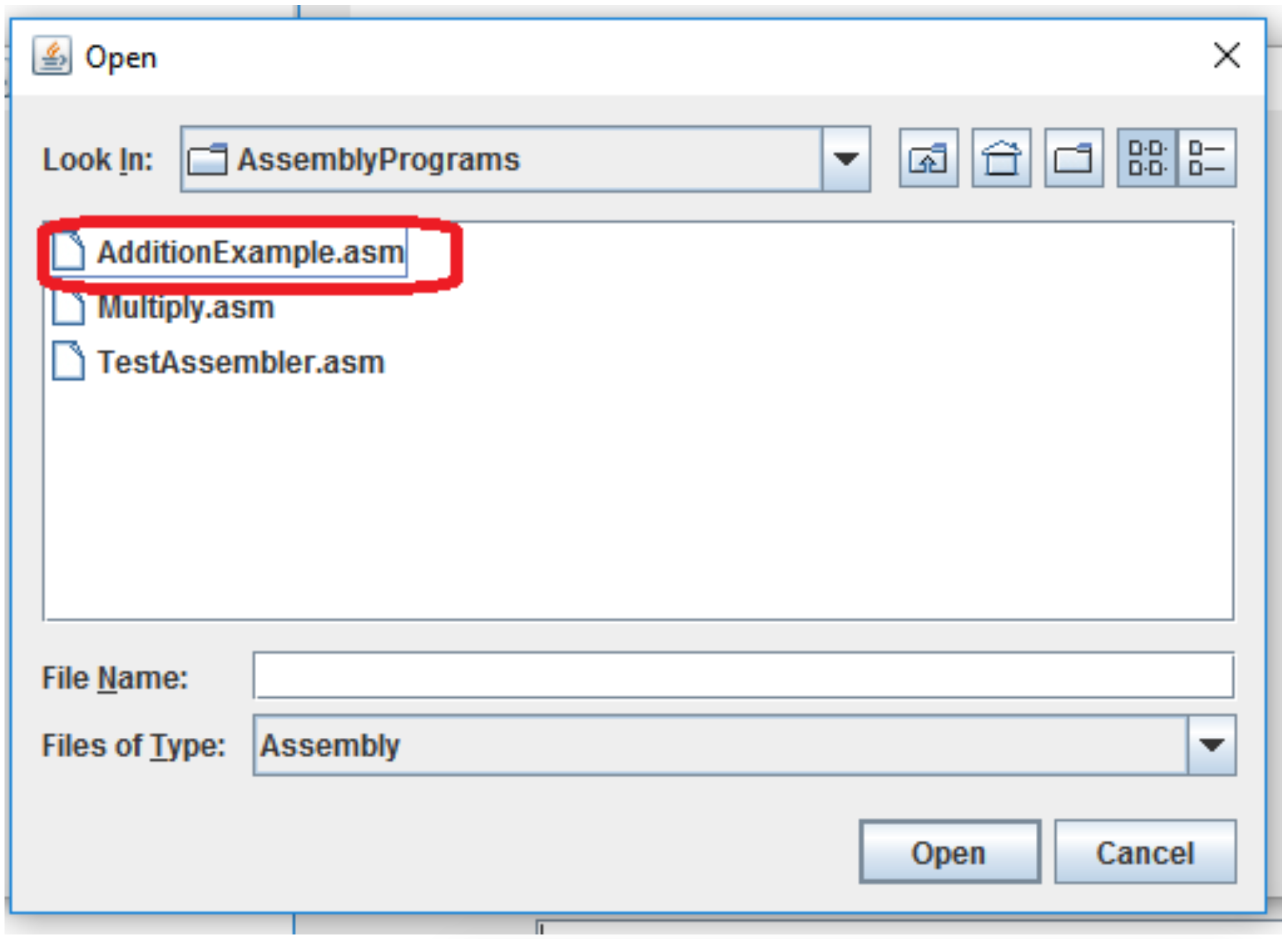
Select the AdditionExample.asm program. This is Program 2.5 from Chapter 2, and adds two values from memory together and stores the result back in memory.
Figure 4-5: Running the assembler - step 3
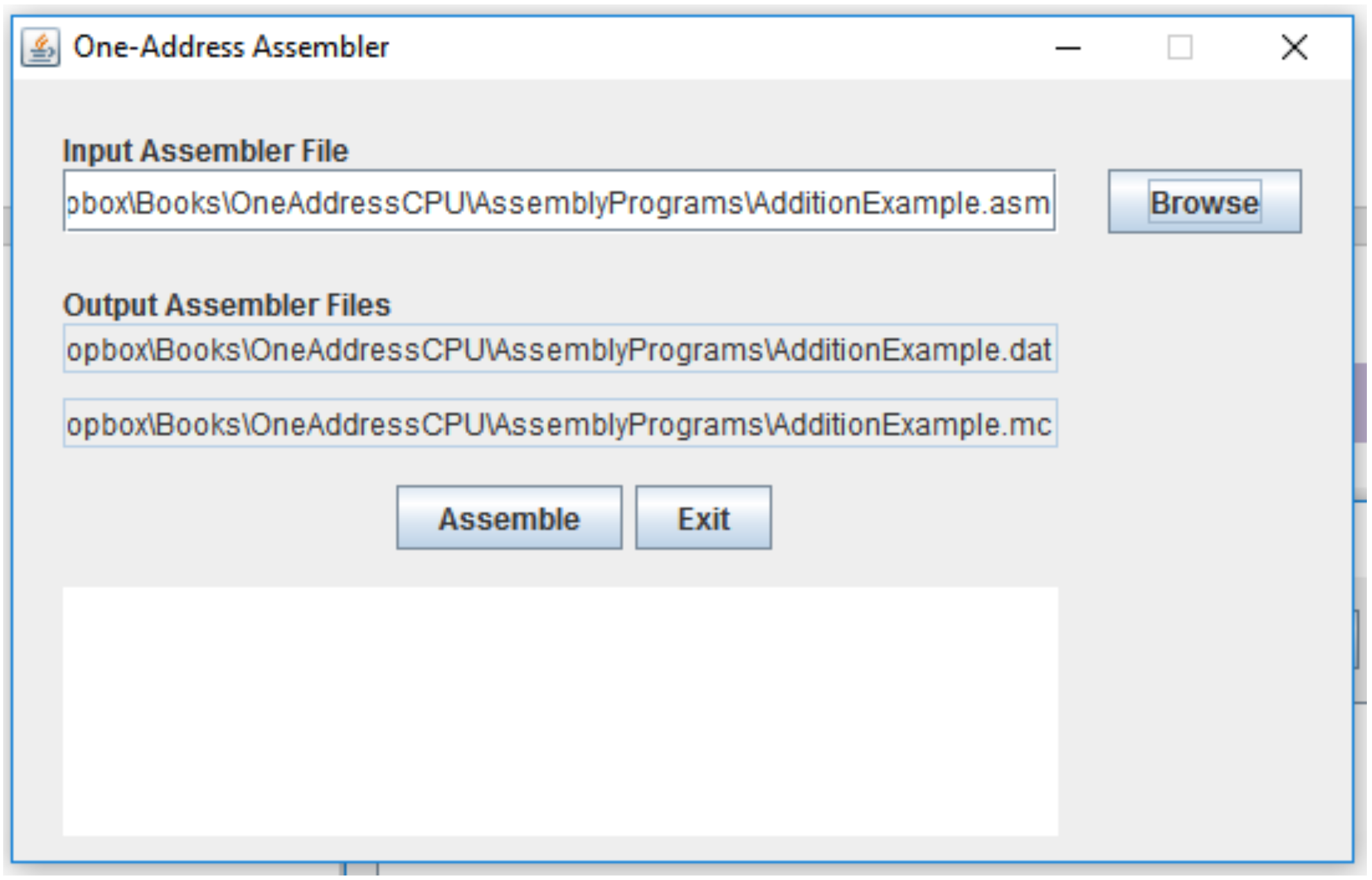
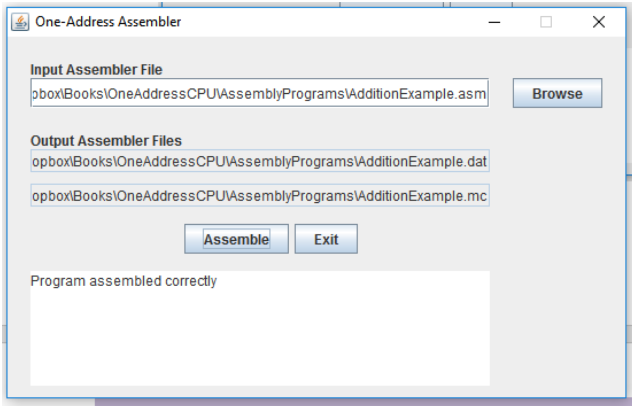
The program will display the following screen, which says that the assembler will use as input the AdditionExample.asm file, and if it successfully completes will produce two output files, AdditionExample.mc (the machine code) and AdditionExample.dat (the data). Click the Assemble button.
Figure 4-6: Running the assembler - step 4
You should get the following message that the assembly completed successfully. Click Exit to close the assembler.
Figure 4-7: Running the assembler - step 5
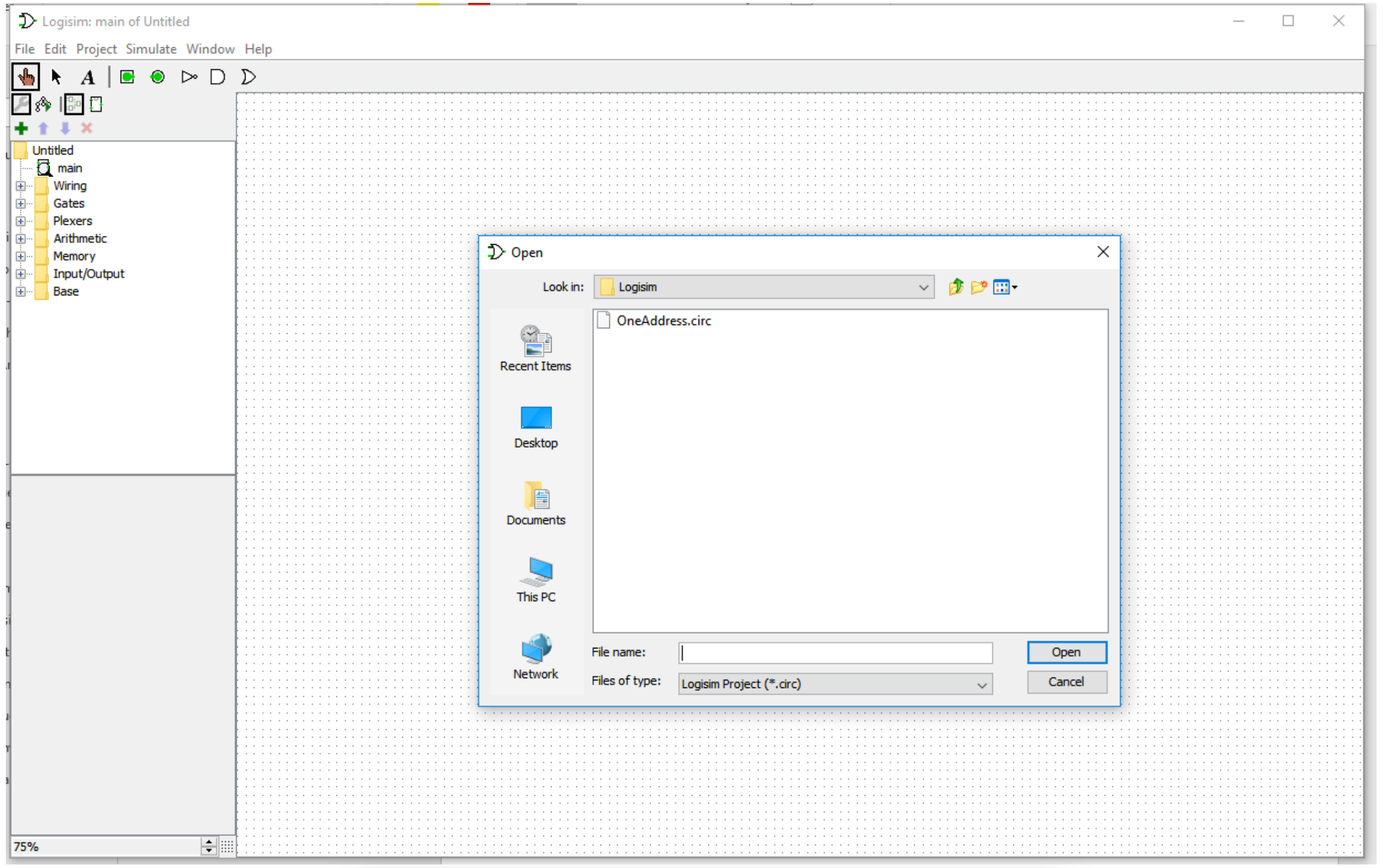
Go to the subdirectory called Logisim, and click on the icon for logisim-generic-2.7.1.jar. This will open Logisim, and you should see the following screen. Choose the File- >Open option, select the Logisim directory, and open the OneAddressCPU.circ file.
Figure 4-8: Running the CPU - step 1
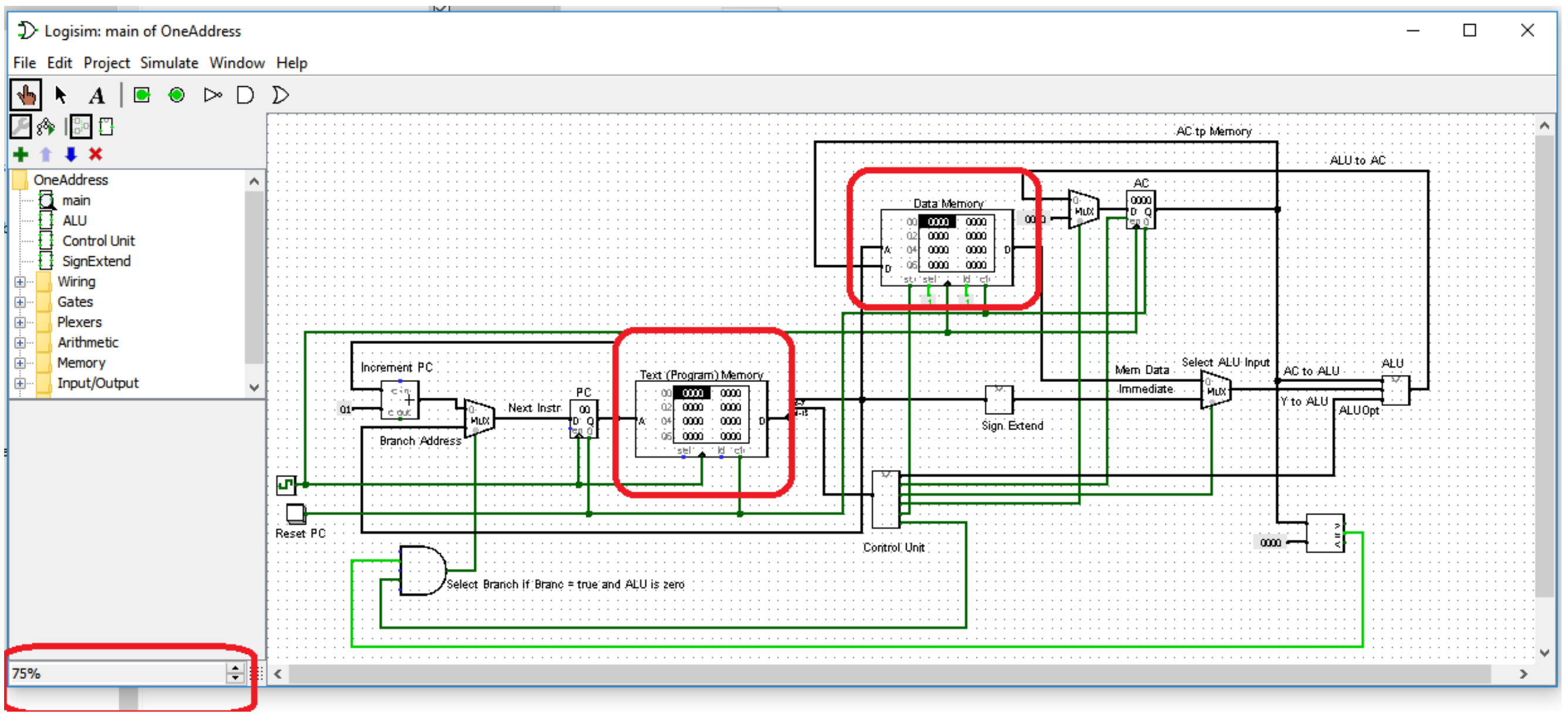
You should now see a screen with the One-Address CPU on it. Set the Zoom size (circled in the picture) to 75% (or 50% if needed) to see the entire diagram. For now the only two areas of the CPU se are interested in are the Text Memory and the Data Memory, which are circled in the diagram.
Figure 4-9 Running the CPU - step 2
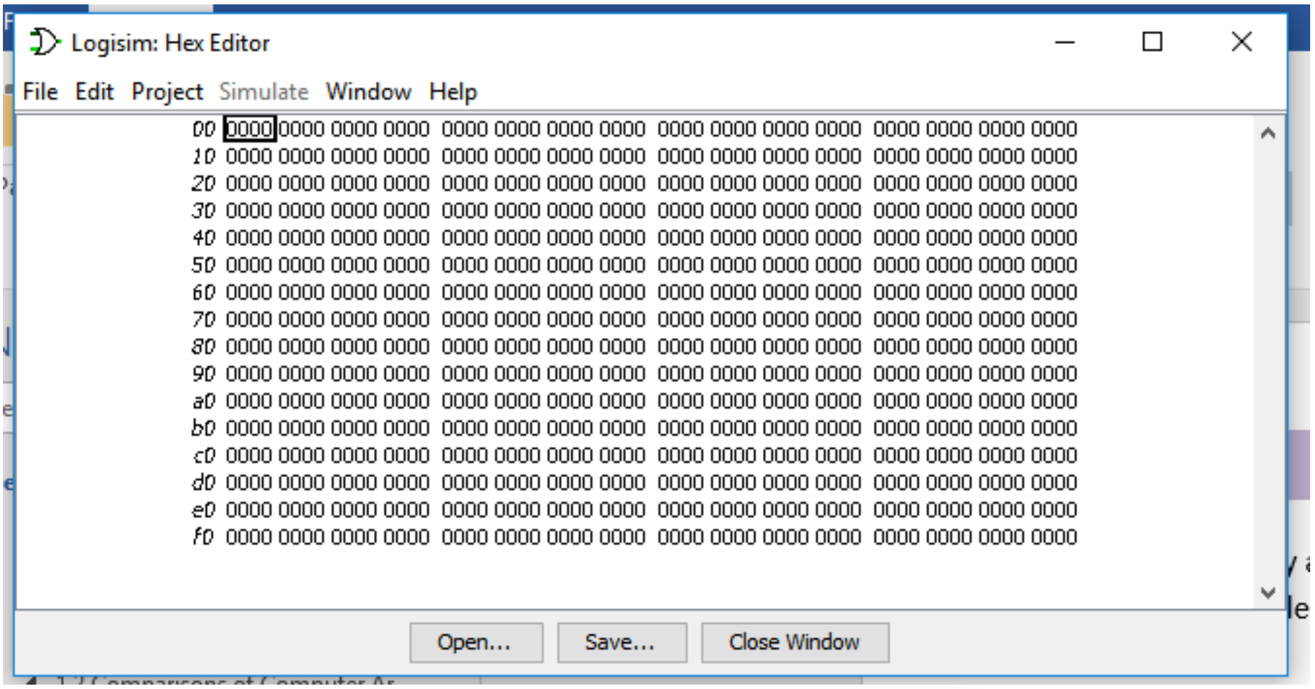
Right click on Text Memory box, and select the Edit Contents option. You should see the following editor for the memory appear on your screen. Note that the input values for this memory are in hexadecimal, but we are going to fill it in from the files that were created by the assembler, and the assembler has written the files in hexadecimal.
Figure 4-10: Running the CPU - step 2
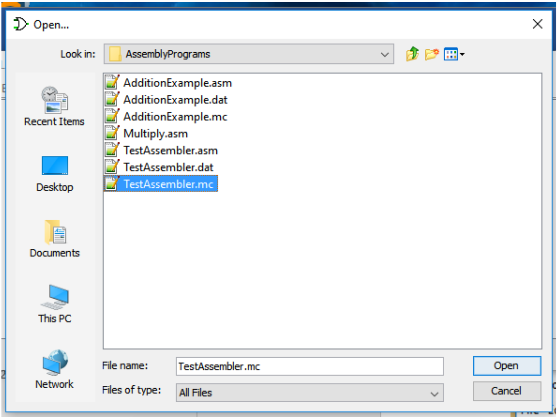
Choose the Open option, go the AssemblyPrograms directory, and select the AdditionExample.mc file.
Figure 4-11: Running the CPU - step 3
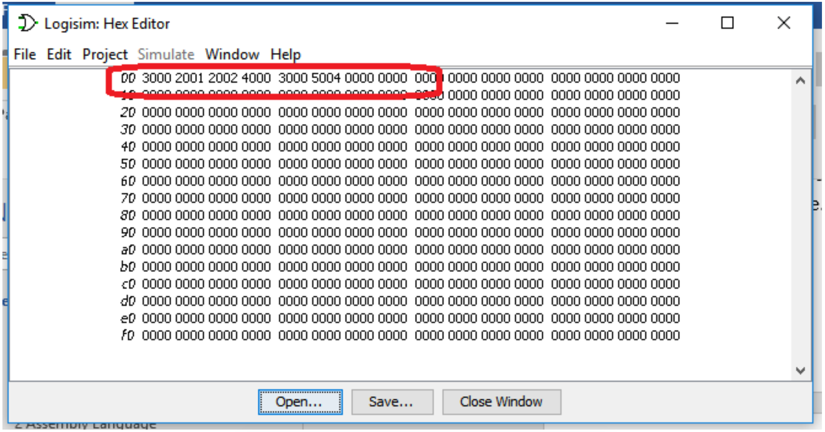
You should now have the AdditionExample machine code in this data block, as in the following example. Select the close option, and the machine code is now available in the CPU.
Figure 4-12: Running the CPU - step 4
Repeat steps 9-11 for the Data Memory using the AdditionExample.dat file. Your data and program memory should now both be initialized.
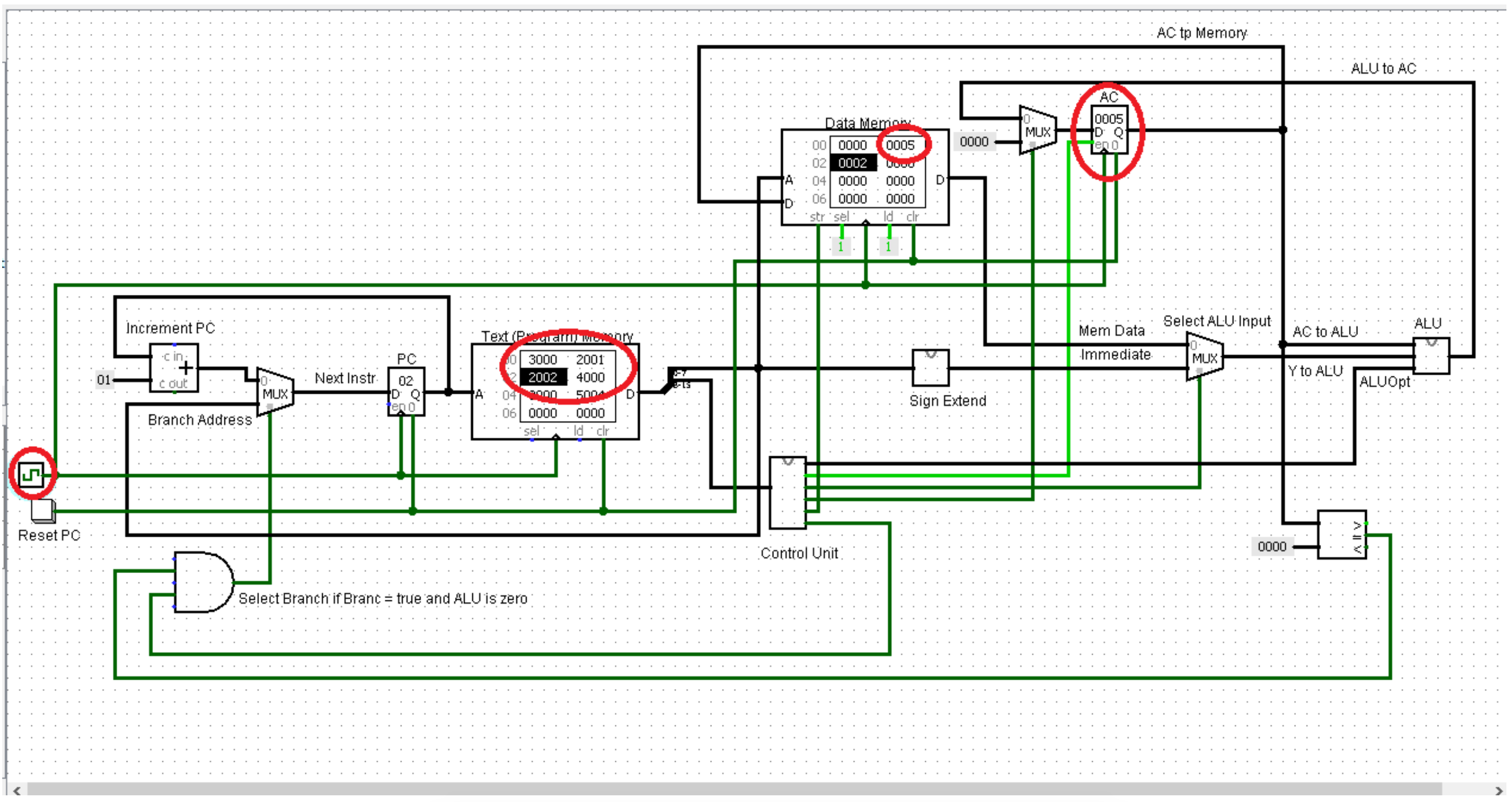
Clicking twice on the clock (remember that the registers and memory only change on a positive edge trigger, not a negative edge trigger), and the clac instruction will execute. This will not result in a change because the $ac is already zero. Click the clock twice more, and you should see program is at instruction 2, and the $ac change to 5.
Figure 4-13: Running the CPU - step 5
Clicking on the clock 6 more times shows that the program has completed, and the value of 7 (5+2) has been calculated and store at memory address 0. The last two instructions, clac and beqz halt, simply put the program in an infinite loop at its end so that it does not continue to execute through the rest of memory.
In Logisim there are a number of ways to control the simulation using the Simulation option. Of particular use is the tick frequency (how often to a clock click happens), tick enabled (which runs the clock at the tick frequency), and Logging (which provides an easy way to review your results).