1.28: The limit that \(V_{0} \rightarrow \infty\) (the infinite square well)

At the walls where the potential is infinite, we see from Equation (1.27.2) that the solutions decay immediately to zero since \(\alpha \rightarrow \infty\). Thus, in the classically forbidden region of the infinite square well \(\psi=0\).

The wavefunction is continuous, so it must approach zero at the walls. A possible solution with zeros at the left boundary is

\[ \psi(x)=A\ sin(k(x+L/2)) \nonumber \]

where k is chosen such that ψ = 0 at the right boundary also:

\[ kL=n\pi \nonumber \]

To normalize the wavefunction and determine A, we integrate:

\[ \int_{-\infty}^{+\infty}|\psi(x)|^{2} d x=\int_{-L / 2}^{L / 2} A^{2} \cos ^{2}(n \pi x / L+n \pi / 2) d x \nonumber \]

From which we determine that

\[ A = \sqrt{2/L} \nonumber \]

The energy is calculated from Equation (1.25.3)

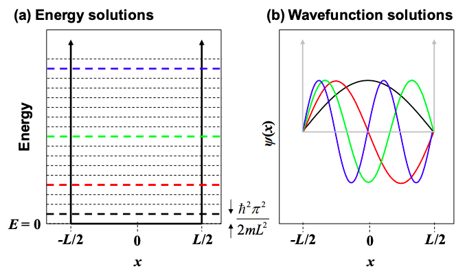
\[ E = \frac{\hbar^{2}k^{2}}{2m}=\frac{\hbar^{2}\pi^{2}n^{2}}{2mL^{2}} \nonumber \]

The first few energies and wavefunctions of electrons in the well are plotted in Figure 1.28.1.

Two characteristics of the solutions deserve comment:

1. The bound states in the well are quantized – only certain energy levels are allowed.
2. The energy levels scale inversely with \(L^{2}\). As the box gets smaller each energy level and the gaps between the allowed energy levels get larger.

Figure \(\PageIndex{1}\): . The lowest four states for a single electron in an infinite square well. Note that we have plotted ψ(x) not \(|ψ(x)|^{2}\).