2.2: How many electrons? Fermi-Dirac Statistics

In the previous section, we determined the allowed energy levels of a particle in a quantum well. Each energy level and its associated wavefunction is known as a "state‟. The Pauli exclusion principle forbids multiple identical electrons from occupying the same state simultaneously. Thus, one might expect that each state in the conductor can possess only a single electron. But electrons also possess spin, a purely quantum mechanical characteristic. For any given orientation, the spin of an electron may be measured to be +1/2 or -1/2. We refer to these electrons as spin up or spin down.

Spin up electrons are different to spin down electrons. Thus the exclusion principle allows two electrons per state: one spin up and one spin down.

Next, if we were to add electrons to an otherwise "empty‟ material, and then left the electrons alone, they would ultimately occupy their equilibrium distribution.

As you might imagine, at equilibrium, the lowest energy states are filled first, and then the next lowest, and so on. At T = 0K, state filling proceeds this way until there are no electrons left. Thus, at T = 0K, the distribution of electrons is given by

\[ f(E,\mu)=u(\mu - E) \nonumber \]

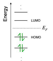
where u is the unit step function. Equation 2.2.1 shows that all states are filled below a characteristic energy, \(\mu\), known as the chemical potential. When used to describe electrons, the chemical potential is also often known as the Fermi Energy, \(E_{F}=\mu\). Here, we will follow a convention that uses \(\mu\) to symbolize the chemical potential of a contact, and \(E_{F}\) to describe the chemical potential of a conductor.

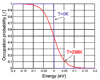
Equilibrium requires that the electrons have the same temperature as the material that holds them. At higher temperatures, additional thermal energy can excite some of the electrons above the chemical potential, blurring the distribution at the Fermi Energy; see Figure 2.2.1.

For arbitrary temperature, the electrons are described by the Fermi Dirac distribution:

\[ f(E,\mu)=\frac{1}{1+\text{exp}[(E-\mu)/kT]} \nonumber \]

Note that Equation 2.2.2 reduces to Equation 2.2.1 at the T = 0K limit. At the Fermi Energy, \(E=E_{F}=\mu\), the states are half full.

Figure \(\PageIndex{1}\): The occupation probability for electrons at two different temperatures. The chemical potential in this example is \(\mu =0\).

It is convenient to relate the Fermi Energy to the number of electrons. But to do so, we need to know the energy distribution of the allowed states. This is usually summarized by a function known as the density of states (DOS), which we represent by g(E). There will be much more about the DOS later in this section. It is defined as the number of states in a conductor per unit energy. It is used to calculate the number of electrons in a material.

\[ n=\int^{+\infty}_{-\infty} g(E)f(E,\mu)dE \nonumber \]

Figure \(\PageIndex{2}\): At left, we show a possible energy structure for a molecule at T = 0K. You can think of a molecule as a little dot that confines electrons in every direction. Thus, like the 1 dimensional quantum well studied previously, the energy levels, or states, in a molecule are discrete. For a molecule each state is often described as a molecular orbital. Below the Fermi energy, each molecular orbital, contains two electrons, one spin up and one spin down. We represent these electrons with upward and downward pointing arrows. The highest occupied molecular orbital is frequently abbreviated as the HOMO. The lowest unoccupied molecular orbital is the LUMO.