2.9: Periodic Boundary Conditions

Usually, our material does not exist in isolation, but rather it may be connected to contacts, for example. So we have a problem: When determining its energy structure, how do we treat the boundaries between our material and the rest of the physical world?

First of all, if the material is big enough (for example, if a quantum wire is long enough), the boundaries will not significantly affect the electron states in the majority of the material. If this is true, we can choose any boundary conditions that are convenient. Indeed, we shall continue for the moment assuming that we can choose convenient boundary conditions. But note that in nanoscale devices, boundary conditions can be problematic; see the previous discussion on 0-d materials coupled to contacts.

When boundaries do not dominate the properties of the material, the usual choice is periodic boundary conditions. As shown in Figure 2.9.1, to apply periodic boundary conditions, we take the wavefunction of the material, and make infinite copies in the unconfined directions. This gives us the ability to analyze electrons traveling in those directions in the material. After all, if just a single, isolated copy of the material was studied, the material could not support traveling electrons, only standing waves.

Figure \(\PageIndex{1}\): Given periodic boundary conditions, only certain k values are allowed in the "unconfined‟ direction of a quantum wire.

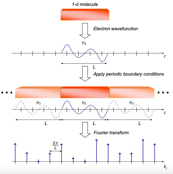
But forcing periodicity in real space affects the Fourier transform of the wavefunction. In k-space, the periodic wavefunction is discrete. For example, on the long axis of a quantum wire of length L, the allowed k-values are spaced by

\[ \Delta k = \frac{2\pi}{L} \nonumber \]

Each allowed k-value corresponds to a plane wave, and each allowed k-value corresponds to a discrete electron wavefunction with a characteristic energy. As we shall see, knowing the separation of k-states in k-space allows us to easily count the number of electron states in the material.

The other way to think about the limitation to certain discrete k values in a periodic material is to recall that any periodic structure supports modes. Consequently, there are only certain allowed wavevectors for delocalized electrons in a periodic molecule. We characterize these modes by their wavevector, k given by \(k = 2\pi n/Na_{0}=2\pi n/L\), where L is the length of the molecule. The allowed k states are therefore:

\[ k = 0, \pm \frac{2\pi}{L}, \pm \frac{4\pi}{L}, \pm\frac{6\pi}{L},… \nonumber \]

Figure \(\PageIndex{2}\): Several modes on a ring. Because the ring is periodic, only the wavevectors, \(k = 2\pi n/L\) give stable states, where L is the perimeter of the ring and n is an integer.

Thus, in a conductor where we have applied periodic boundary conditions, the spacing of the allowed k states is determined by the length of conductor.