3.8: Analytic calculations of the effects of charging

The most accurate method to determine the IV characteristics of a quantum dot device is to solve for the potential and the charge density following the scheme of Figure 3.7.4. This is often known as the self consistent approach since the calculation concludes when the initial guess for the potential U has been modified such that it is consistent with the value of U calculated from the charge density.

Unfortunately, numerical approaches can obscure the physics. In this section we will make some approximations to allow an analytic calculation of charging. We will assume operation at T = 0K, and discrete molecular energy levels, i.e. weak coupling between the molecule and the contacts such that \((\Gamma = \hbar/\tau) \rightarrow 0\).

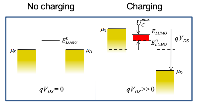
Let's consider a LUMO state with energy \(E_{\text{LUMO}}\) that is above the equilibrium Fermi level. Under bias, the energy of the LUMO is altered by electrostatic and charginginduced changes in potential. When we apply the drain source potential, it is convenient to assume that the molecule is ground. Under this convention, the only change in the molecule‟s potential is due to charging. Graphically, the physics can be represented by plotting the energy level of the molecule in the presence and absence of charging. In Figure 3.8.1, below, we shade the region between the charged and uncharged LUMOs. Now

\[ U_{C} = \frac{q^{2}}{C_{ES}}(N-N_{0}) , \nonumber \]

and at T = 0K, \(N_{0}=0\) for the LUMO in Figure 3.8.1. Thus, the area of the shaded region is proportional to the charge on the molecule.

Figure \(\PageIndex{1}\): Under bias, the energy levels of the molecule can be shifted by electrostatic and charging-induced changes in the potential. If we assume the molecule is ground, then the electrostatic changes in potential alter the source and the drain. Only charging then alters the molecular energy level. The difference between the charged and uncharged molecular energy levels is proportional to the charge on the molecule and is shaded red.

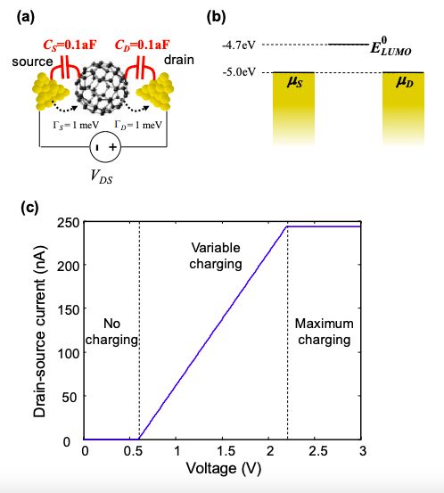
The graphical approach is a useful guide to the behavior of the device. There are three regions of operation, each shown below.

Figure \(\PageIndex{2}\): The three regions of operation for a two terminal quantum dot device with discrete energy levels at T = 0K. Current flow requires the source to inject carriers into the molecular energy levels. The onset of current flow occurs when the chemical potential of the source is resonant with the LUMO. Additional drain-source bias charges the molecule, and the current increases linearly with the molecular charge. Finally, a maximum charge density is reached. Further increases in applied bias do not increase the charging energy or the current flow.

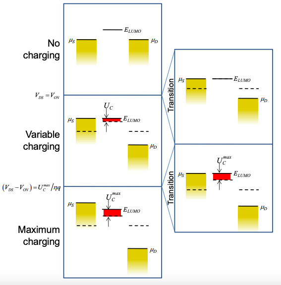
No charging

At T = 0K and \(V_{DS}=0\) there is no charge in the LUMO. Charging cannot occur unless electrons can be injected from the source into the LUMO. So as \(V_{DS}\) increases, charging remains negligible until the LUMO energy is aligned with the chemical potential of the source. Thus, for \(\mu_{S} < E_{\text{LUMO}}\) the charging energy, \(U_{C} = 0\).

In this region, \(I_{DS}=0\). We define the bias at which current begins to flow as \(V_{DS}=V_{ON}\). \(V_{ON}\) is given by

\[ V_{ON}=\frac{E^{0}_{\text{LUMO}} -\mu_{S}}{q\eta} \nonumber \]

where \(E^{0}_{\text{LUMO}}\) is the LUMO energy level at equilibrium.

Maximum charging

For \(\mu_{S} > E_{\text{LUMO}}\), the charge on the LUMO is independent of further increases in \(V_{DS}\). It is a maximum. From Equation (3.7.8), the LUMO's maximum charge is

\[ N^{\text{max}}=\frac{2\tau_{D}}{\tau_{S}+\tau_{D}} \nonumber \]

Consequently, the charging energy is

\[ U^{\text{max}}_{C} = \frac{2q^{2}}{C_{ES}} \frac{\tau_{D}}{\tau_{S}+\tau_{D}} \nonumber \]

For all operation in forward bias, it is convenient to calculate the current from Equation (3.7.6). At T = 0K, the charges injected by the drain \(N_{D} = 0\). Consequently,

\[ I_{DS}=\frac{qN^{max}}{\tau_{D}}=\frac{2q}{\tau_{S}+\tau_{D}} \nonumber \]

Maximum charging occurs for voltages \(\mu_{S} > E_{\text{LUMO}}\). We can rewrite this condition as

\[ (V_{DS}-V_{ON}) > U_{C}^{max}/\eta q \nonumber \]

Variable charging

Charging energies between \(0 < U_{C} < U_{C}^{max}\) require that \(\mu_{S} = E_{\text{LUMO}}\). Assuming that the molecule is taken as the electrostatic ground, then \(\mu_{S} = E_{\text{LUMO}} = U_{C}\) for this region of operation. Calculating the current from Equation (3.7.6) gives

\[ I_{DS}=\frac{qN}{\tau_{D}} \nonumber \]

Then, given that \(U_{C}=q^{2}N/C_{ES}\), we can rearrange Equation (3.8.7) to get

\[ I_{DS} = \frac{C_{ES}U_{C}}{q\tau_{D}} \nonumber \]

Then, from Equations (3.6.3) and (3.6.4) and noting that \(\mu_{S}=E_{\text{LUMO}} = U_{C}\),

\[ I_{DS} = \frac{C_{ES}}{\tau_{D}}\eta (V_{DS}-V_{ON}) . \nonumber \]

This region is valid for voltages

\[ 0 < (V_{DS}-V_{ON}) < U_{C}^{max}/\eta q . \nonumber \]

The full IV characteristic is shown below. Under our assumptions the transitions between the three regions of operation are sharp. For T > 0K and \((\Gamma = \hbar/\tau) > 0\) these transitions are blurred and are best calculated numerically; see the Problem Set.

Figure \(\PageIndex{3}\): (a) An example of a single molecule device subject to strong charging effects. The coupling between the molecule and the contacts is small relative to the applied voltage, i.e. \(\Gamma_{S}/q=\Gamma_{D}/q=1\ mV\). The source and drain capacitances yield a large charging potential per electron \(q^{2}/C_{ES}=0.8\ eV\). The voltage division factor is \(\eta=0.5\). (b) The offset between the LUMO and the contact work functions is 0.3 eV, consequently, \(V_{ON}=0.3/\eta=0.6V\) (c) The current-voltage characteristic.