4.6: The Quantum Limit of Conductance
- Page ID
- 50034

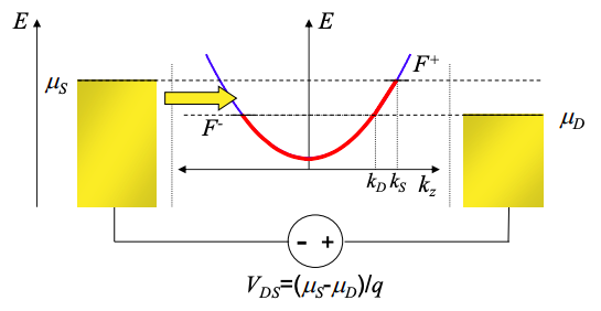
We've seen that in a quantum wire, current flow requires a difference in the quasi Fermi levels for electrons moving with and against the current. Furthermore, only electrons between the quasi Fermi levels, i.e. \(F^{-}<E<F^{+}\) carry current.
In general, the total current in a quantum wire is
\[ I = qN/\tau \nonumber \]
where N is the number of uncompensated electrons, and \(\tau\) is their transit time (the time they take to cross from one end of the wire to the other). Let‟s use Equation (4.6.1) to calculate the current in a single mode quantum wire at T=0K.
The velocity of electrons in the wire is given by the group velocity (see Problem 3)
\[ v = \frac{1}{\hbar}\frac{dE}{dk} \nonumber \]
As an aside, we note that if \(F^{+}-F^{-}\) is small, the current carrying electrons all move at approximately the equilibrium Fermi velocity.
\[ v_{F}=\left.\frac{1}{\hbar} \frac{d E}{d k}\right|_{E_{F}} \nonumber \]
The transit time in Equation (4.6.1) is related to the length of the wire, L, and the velocity of the uncompensated electrons:
\[ \tau = \frac{L}{v} = L / \left( \frac{1}{\hbar} \frac{dE}{dk}\right) \nonumber \]
The number of uncompensated electrons is equal to the number of electrons in the states \(k_{D} < k < k_{S}\), equivalent to \(\mu_{D} < E < \mu_{S}\) in Figure 4.6.1. Each k state occupies \(\Delta k = 2\pi / L\). Recall also that there are two electrons per k state (one of each spin). Thus,
\[ N = 2 \int^{k_{S}}_{k_{D}} \frac{dk}{2\pi / L} \nonumber \]
Equation (4.6.1) is then
\[ I = 2q \int^{k_{S}}_{k_{D}} \frac{dk}{2\pi /L} \frac{1}{h L}\frac{dE}{dk} \nonumber \]
Simplifying gives
\[ I = \frac{2q}{h} \int^{k_{S}}_{k_{D}} dk\ \frac{dE}{dk} \nonumber \]
Changing the variable of integration to energy gives
\[ I = \frac{2q}{h} \int^{\mu_{S}}_{\mu_{D}} dE \nonumber \]
\( =\frac{2q}{h} (\mu_{S}-\mu_{D}) \)
Note \(V_{DS} = -(\mu_{D}-\mu_{S})/q\), thus
\[ I=\frac{2q^{2}}{h} V \nonumber \]
This expression demonstrates that the resistance of an ideal single mode wire is
\[ R = \frac{h}{2q^{2}} \approx 12.9\ k\Omega \nonumber \]
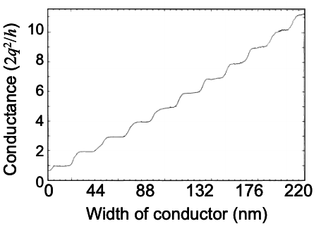
A multiple mode wire with M modes can be thought of as M single mode wires in parallel. Since parallel conductances add, the quantum limit is usually written as a conductance. For a multimode ballistic wire the conductance is
\[ G_{C} = \frac{2q^{2}}{h}\ M \nonumber \]
This is the famous quantum limited conductance. It yields the surprising conclusion that even ballistic conductors have a resistance, although this resistance is independent of the length of the conductor.
But a resistance implies that power is dissipated when a current flows. Given that electron transport in the wire is ballistic, where do the resistive power losses occur?
If we look at Figure 4.6.1 we find that carriers entering the wire from the source propagate without change in potential until they reach the drain where they must come to equilibrium at chemical potential \(\mu_{D}\). Thus, the power is dissipated in the drain.
The quantum limit in conductance arises as a consequence of the interface between the contact with its (ideally) infinite modes and infinite number of electrons all at equilibrium, and a conductor with a small number of modes supporting non-equilibrium electrons. Thus, the quantum limit can be thought of as a contact resistance.
Of course, as the number of modes in the conductor increases, the contact resistance decreases. In the classical limit, it can be completely ignored.