4.12: Effective Mass

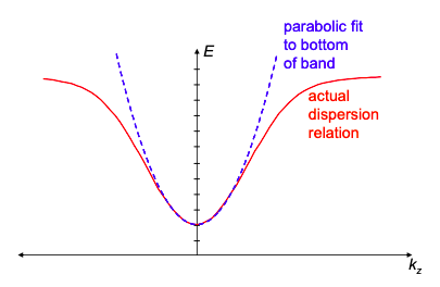
So far, both the classical and quantum models of conduction have assumed that the current carrying electrons occupy pure planewave states. The dispersion relation of real materials, however, varies from the ideal parabola. We can approximate any dispersion relation by a plane wave if we allow the mass of the electron to vary. We call the modified mass the effective mass. Under this approximation, the electron is thought of as a classical particle and various complex phenomena are wrapped up in the effective mass. For example, given dispersion relation E(k), a Taylor expansion about k = 0 yields:

\[ \left. E(k) = E(0)+k\frac{dE}{dk} \right|_{k=0} \left. + \frac{1}{2}k^{2}\frac{d^{2}E}{dk^{2}} \right|_{k=0} + … \nonumber \]

Approximating the dispersion relation by a plane wave gives

\[ E(k) = E_{0} + \frac{\hbar^{2}k^{2}}{2m^{*}} \nonumber \]

Equating the quadratic terms in Eqations. (4.13.1) and (4.13.2) we get an expression for the effective mass

\[ m^{*} = \hbar^{2}\left( \frac{d^{2}E}{dk^{2}} \right)^{-1} \nonumber \]

The effective mass concept is commonly used in classical models of electron transport, especially models of mobility like Equation (4.12.2).

Figure \(\PageIndex{1}\): We can model conduction in a material of arbitrary dispersion relation by assuming plane wave electron states with variable (effective) electron mass, m*, obtained by fitting a parabola to the bottom of the band.