5.10: The Ballistic Quantum Wire FET

Last updated
Save as PDF

Page ID: 51621

Marc Baldo
Massachusetts Institute of Technology via MIT OpenCourseWare

\( \newcommand{\vecs}[1]{\overset { \scriptstyle \rightharpoonup} {\mathbf{#1}} } \) \( \newcommand{\vecd}[1]{\overset{-\!-\!\rightharpoonup}{\vphantom{a}\smash {#1}}} \)\(\newcommand{\id}{\mathrm{id}}\) \( \newcommand{\Span}{\mathrm{span}}\) \( \newcommand{\kernel}{\mathrm{null}\,}\) \( \newcommand{\range}{\mathrm{range}\,}\) \( \newcommand{\RealPart}{\mathrm{Re}}\) \( \newcommand{\ImaginaryPart}{\mathrm{Im}}\) \( \newcommand{\Argument}{\mathrm{Arg}}\) \( \newcommand{\norm}[1]{\| #1 \|}\) \( \newcommand{\inner}[2]{\langle #1, #2 \rangle}\) \( \newcommand{\Span}{\mathrm{span}}\) \(\newcommand{\id}{\mathrm{id}}\) \( \newcommand{\Span}{\mathrm{span}}\) \( \newcommand{\kernel}{\mathrm{null}\,}\) \( \newcommand{\range}{\mathrm{range}\,}\) \( \newcommand{\RealPart}{\mathrm{Re}}\) \( \newcommand{\ImaginaryPart}{\mathrm{Im}}\) \( \newcommand{\Argument}{\mathrm{Arg}}\) \( \newcommand{\norm}[1]{\| #1 \|}\) \( \newcommand{\inner}[2]{\langle #1, #2 \rangle}\) \( \newcommand{\Span}{\mathrm{span}}\)\(\newcommand{\AA}{\unicode[.8,0]{x212B}}\)

Consider the ballistic quantum wire FET shown in Figure 5.10.1.

Screenshot 2021-05-18 at 19.06.20.png — Figure \(\PageIndex{1}\): A quantum wire FET. The gate is wrapped around the wire to maximize the capacitance between the channel and the gate. The length of the wire is L = 100nm, the gate capacitance is \(C_{G}\) = 50 aF per nanometer of wire length, and the electron mass, m, in the wire is \(m=m_{0}=9.1\times10^{-31} kg\).

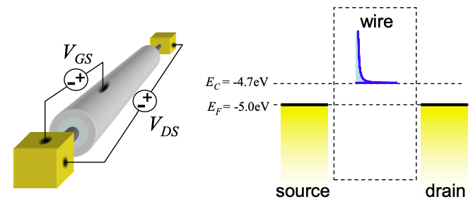
We will assume that there is only one parabolic band in the wire.

From Equation (2.10.6), the density of states in the wire is:

Screenshot 2021-05-18 at 19.10.38.png — Figure \(\PageIndex{2}\): The bandstructure and density of states in a single mode quantum wire.

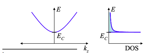
\[ g(E)dE=\frac{2L}{h}\sqrt{\frac{2m}{E-E_{C}}}u(E-E_{C})dE , \nonumber \]

where L is the length of the wire, and m is the electron mass in the wire. But only half of these states contain electrons traveling in the positive direction. Thus, we must divide Equation (5.10.1) by two to yield:

\[ g^{+}(E)dE=\frac{1}{2}\times\frac{2L}{h}\sqrt{\frac{2m}{E-E_{C}}}u(E-E_{C})dE \nonumber \]

Given the position of the Fermi Energy, this band is the conduction band. We will label the energy at the bottom of the conduction band, \(E_{C}\). Since we model electrons moving along the wire as plane waves, within the parabolic band we have

\[ E-E_{C} =\frac{\hbar^{2}k^{2}}{2m} = \frac{1}{2}mv^{2} \nonumber \]

We can rewrite Equation (5.10.2) in terms of the velocity, v, of the electron:

\[ g^{+}(E)dE = \frac{1}{2}\times \frac{4L}{hv(E)}u(E-E_{C})dE \nonumber \]

Now L/v is the transit time of an electron through the wire, thus

\[ g^{+}(E)dE = \frac{1}{2}\times \frac{4\tau(E)}{h}u(E-E_{C})dE \nonumber \]

We can substitute Equation (5.10.5) into the expression for the current density (Equation (5.9.4)) to obtain

\[ I= \frac{2q}{h}\int^{+\infty}_{-\infty} u(E-E_{C}-U)(f(E,\mu_{S})-(f(E,\mu_{D}))dE . \nonumber \]

\(^{†}\) This analysis of the ballistic quantum wire FET was introduced to me by Mark Lundstrom at Purdue University. For a complete reference see Mark Lundstrom and Jing Guo, "Nanoscale Transistors: Physics, Modeling, and Simulation‟, Springer, New York, 2006.