6.2: Atoms to Molecules

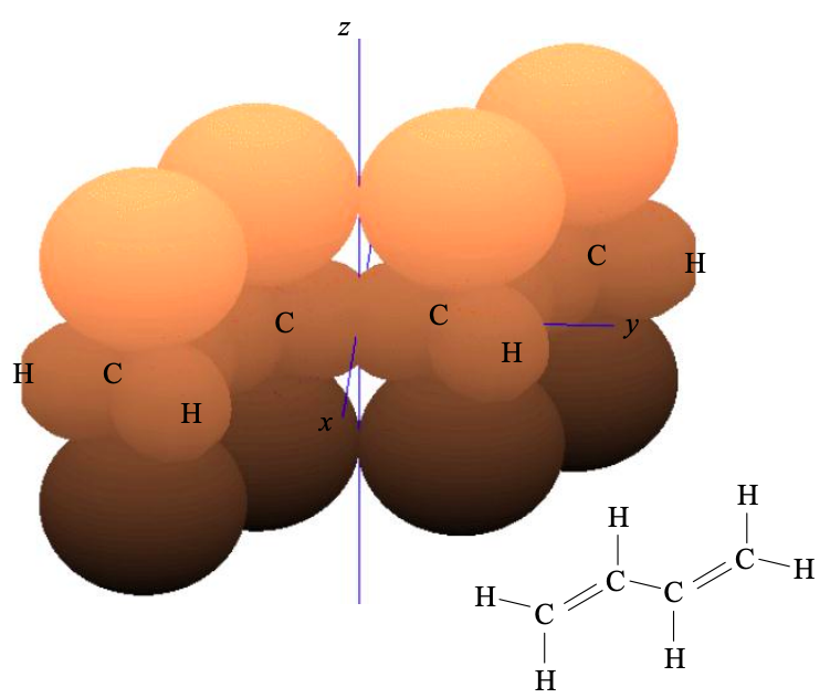
We now seek to determine the electronic states of whole molecules – molecular orbitals. Although we will begin with relatively small molecules, the calculation techniques that we will introduce can be extended to larger materials that we don‟t usually think of as molecules: like Si crystals, for example.

Figure \(\PageIndex{1}\): The molecule 1,3-butadiene. Clouds of electron probability density are shown around each atom. They combine to form molecular orbitals.

In the previous discussion of atomic orbitals, we implicitly assumed that the nucleus is stationary. This is an example of the Born-Oppenheimer approximation, which notes that the mass of the electron, \(m_{e}\), is much less than the mass of the nucleus, \(m_{N}\). Consequently, electrons respond almost instantly to changes in nuclear coordinates.

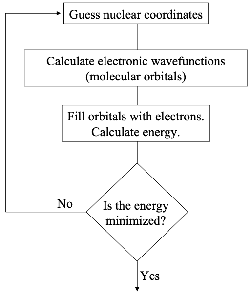
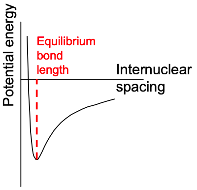
In calculations of the electronic structure of molecules, we have to consider multiple electrons and multiple nuclei. We can simplify the calculation considerably by assuming that the nuclear positions are fixed. The Schrödinger equation is then solved for the electrons in a static potential; see Appendix 3. Different arrangements of the nuclei are chosen and the solution is optimized.

Figure \(\PageIndex{2}\): Technique for calculating the electronic structure of materials.

Figure \(\PageIndex{3}\): The equilibrium internuclear spacing (bond length) in a molecule results from competition between a closerange repulsive force typically with exponential dependence on intermolecular spacing, and a longer-range attractive Coulomb force. Typically the molecular orbitals must be calculated for each internuclear spacing. The energy minima is the equilibrium bond length. Calculating the electronic states for fixed nuclear coordinates is an example of the Born-Oppenheimer approximation.