6.7: Examples of tight binding calculations
- Page ID
- 52281
Let's consider a conductor consisting of four atoms, each of which provides a frontier atomic orbital containing a single electron. A molecular equivalent to this model conductor is 1,3-butadiene; see Figure 6.8.1. Here each carbon atom contributes one electron in a frontier atomic orbital.
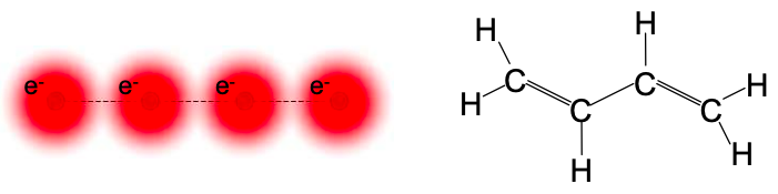
We'll ignore the hydrogen atoms, since the frontier electrons are donated by the carbon atoms. Let's label the four carbon frontier atomic orbitals \(\phi_{1}, \phi_{2}, \phi_{3},\text{ and } \phi_{4}\).
Following Equation (6.4.1), we let the molecular orbitals be
\[ \psi = c_{1}\phi_{1}+c_{2}\phi_{2}+c_{3}\phi_{3}+c_{4}\phi_{4} \nonumber \]
where the \(c_i\) coefficients are yet to be determined.
Let's next consider integrals of the form:
\[ \left< \phi_{m}|H|\psi \right> = \left< \phi_{m}|E|\psi \right> = E \left< \phi_{m}|\psi \right> \nonumber \]
Considering \(m = 1\), \(m=2\), \(m=3\) and \(m=4\) in turn, we get four equations:
\[\begin{align*} \left< \phi_{1}|H|\psi \right> &= c_{1}\alpha_{1} + c_{2}\beta_{12} = c_{1}E \\[4pt]
\left< \phi_{2}|H|\psi \right> &= c_{2}\alpha_{2} + c_{1}\beta_{21}+c_{3}\beta_{23} = c_{2}E \\[4pt]
\left< \phi_{3}|H|\psi \right> &= c_{3}\alpha_{3} + c_{2}\beta_{32}+c_{4}\beta_{34} = c_{3}E \\[4pt]
\left< \phi_{4}|H|\psi \right> &= c_{4}\alpha_{4} + c_{3}\beta_{43} = c_{4}E \end{align*} \nonumber \]
You can think of each equation as describing the interactions between a particular carbon atom, and itself and its neighbors. Solving these equations gives the coefficients \(c_{1}, c_{2}, c_{3}, \text{ and } c_{4}\). To simplify, we will assume that the self energy at each carbon atom is the same, i.e.
\[ \alpha = \alpha_{1} = \alpha_{2}= \alpha_{3}= \alpha_{4} \nonumber \]
In addition, we will assume that the hopping interactions between neighboring carbon atoms are the same, i.e.
\[ \beta = \beta_{12} =\beta_{21} =\beta_{23} =\beta_{32}=\beta_{34}=\beta_{43} \nonumber \]
Perhaps the best way to solve the equations systematically is via a matrix. The equations can be re-written:
\[ \left(\begin{array}{cccc}
\alpha & \beta & 0 & 0 \\
\beta & \alpha & \beta & 0 \\
0 & \beta & \alpha & \beta \\
0 & 0 & \beta & \alpha
\end{array}\right)\left(\begin{array}{l}
c_{1} \\
c_{2} \\
c_{3} \\
c_{4}
\end{array}\right)=E\left(\begin{array}{l}
c_{1} \\
c_{2} \\
c_{3} \\
c_{4}
\end{array}\right) \nonumber \]
This equation is of the familiar form
\[ H| \psi \big \rangle = E| \psi \big \rangle \nonumber \]
where the Hamiltonian is in the form of a matrix, and the wavefunction is a column vector containing the coefficients that weight the atomic orbitals:
\[ H=\left(\begin{array}{cccc}
\alpha & \beta & 0 & 0 \\
\beta & \alpha & \beta & 0 \\
0 & \beta & \alpha & \beta \\
0 & 0 & \beta & \alpha
\end{array}\right), \quad \psi=\left(\begin{array}{l}
c_{1} \\
c_{2} \\
c_{3} \\
c_{4}
\end{array}\right) \nonumber \]
Expressing the Hamiltonian and wavefunction in this form is an example of matrix mechanics, a version of quantum mechanics formulated by Werner Heisenberg that is convenient for many problems. Apart from this example, we won't pursue matrix mechanics in this class.
But it‟s worth taking a moment to examine the structure of the Hamiltonian matrix. Each row now describes the interactions between frontier orbitals on a carbon atom, and itself and its neighbors. The diagonal of the matrix contains the self-energies, and the offdiagonal elements are the hopping interactions. This particular example is tridiagonal, i.e. the matrix elements are zero, except for the diagonal, and its immediately adjacent matrix elements. Linear molecules with alternating single and double bonds always possess tridiagonal matrices.
After a bit of practice with tight binding calculations you should be able to skip directly to writing down the Hamiltonian matrix. For example, consider cyclobutadiene; shown below.
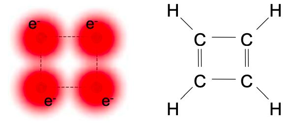
Because of its ring structure, cyclobutadiene has additional hopping interactions between the carbons #1 and #4 that were on the ends of the chain in 1,3-butadiene. These interactions at the 1,4 and 4,1 positions are labeled in red in Equation (6.8.9) below
\[ H=\left(\begin{array}{cccc}
\alpha & \beta & 0 & \textcolor{red}{\beta} \\
\beta & \alpha & \beta & 0 \\
0 & \beta & \alpha & \beta \\
\textcolor{red}{\beta} & 0 & \beta & \alpha
\end{array}\right) \nonumber \]
As you can probably imagine, for all but the simplest molecules, these matrices can get extremely large and unwieldy. And solving them can be extremely computationally intensive. In fact, tight binding calculations are almost never done by hand. But some insight can be gained by analytically solving simple linear molecules.
Returning to 1,3-butadiene, rearranging Equation (6.8.6), we get:
\[ \left(\begin{array}{cccc}
\alpha-E & \beta & 0 & 0 \\
\beta & \alpha-E & \beta & 0 \\
0 & \beta & \alpha-E & \beta \\
0 & 0 & \beta & \alpha-E
\end{array}\right)\left(\begin{array}{l}
c_{1} \\
c_{2} \\
c_{3} \\
c_{4}
\end{array}\right) = 0 \nonumber \]
To find the non-trivial solution (i.e. solutions other than \(c_{1} = c_{2} = c_{3} = c_{4} =0\)) we take the determinant:
\[ \left|\begin{array}{cccc}
\alpha-E & \beta & 0 & 0 \\
\beta & \alpha-E & \beta & 0 \\
0 & \beta & \alpha-E & \beta \\
0 & 0 & \beta & \alpha-E
\end{array}\right|=0 \nonumber \]
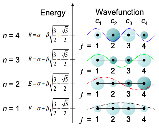
The solutions are:
\[E = \alpha \pm \beta\sqrt{\frac{3}{2}\pm\frac{\sqrt{5}}{2}} \nonumber \]
And the eigenfunctions are:
\[ c_{j} = sin\left(\ jn \frac{\pi}{5} \right), \ \ j,n=1,2,3,4 \nonumber \]
These solutions are summarized in Figure \(\PageIndex{3}\). The molecular orbitals are similar to the standing waves expected for a particle in a box.