6.17: Tight Binding Calculations in Periodic molecules and crystals

Polyacetylene (average bond model)

We now repeat the polyacetylene calculation, but this time we impose periodic boundary conditions and assume molecular wavefunctions of the Bloch form. The solutions are almost identical to the previous calculation in the absence of periodic boundary conditions, but there are some subtle yet important differences in the dispersion relation.

The unit cell of polyacetylene under the average bond model has only a single carbon atom. Let the wavefunction of the jth unit cell be \(\phi(j)\), defined as the frontier atomic orbital of carbon. Since polyacetylene is periodic, we use a Bloch function to describe the molecular orbitals

\[ \psi(x) = \sum_{j}e^{i\frac{2\pi n}{N}j} \phi (x-ja_{0}) \nonumber \]

To derive the energy levels consider \(\left< \phi_{j}|H|\psi(x) \right>\). Now,

\[ \left< \phi_{j}|H|\psi(x) \right> =\epsilon \left< \phi_{j}|\psi(x) \right> \nonumber \]

Under the tight binding approximation, this simplifies to

\[ \beta\ \text{exp}\left[ i \frac{2\pi n}{N}(j-1) \right] + \alpha\ \text{exp}\left[ i \frac{2\pi n}{N} j\right] +
\beta\ \text{exp}\left[ i \frac{2\pi n}{N} (j+1)\right] = \epsilon\ \text{exp}\left[ i \frac{2\pi n}{N} j\right] \nonumber \]

where \(\beta = \left< \phi_{j}|H|\phi_{j+1} \right>\) and \(\alpha = \left< \phi_{j}|H|\phi_{j} \right>\).

Simplifying gives (compare Equation (6.9.4))

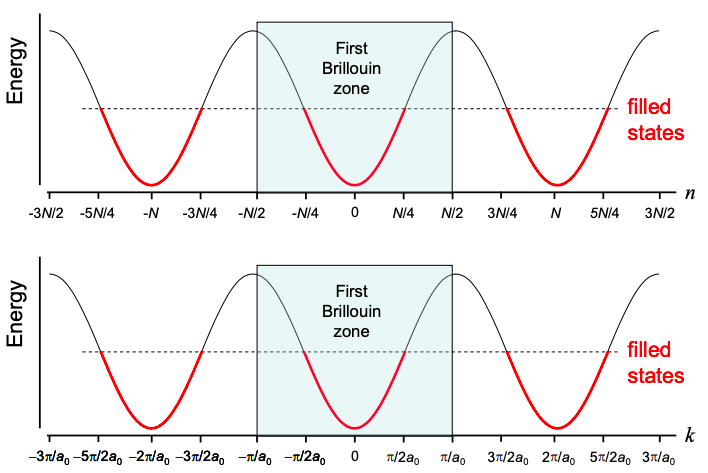
\[ \epsilon_{n}=\alpha+2\beta\ cos\frac{2\pi n}{N} \nonumber \]

Re-writing Equation (6.18.4) gives

\[ \epsilon_{k}=\alpha+2\beta\ cos\ ka_{0} \nonumber \]

where

\[ k =\frac{2\pi n}{Na_{0}} = \frac{2\pi n}{L} \nonumber \]

Once again, we note that each carbon atom contributes a single electron to its frontier orbital, thus for a N-repeat polymer, there are N electrons.

We can determine whether polyacetylene is a metal or insulator by counting k states. The spacing between k states is \(2\pi /L\). Thus in the first Brillouin zone, there must be \(2\pi /a_{0}\ / \ 2\pi /L = L/a_{0} = N\) states. But each molecular orbital holds two electrons, one of each spin. Filling the lowest energy states first, only the first N/2 k states are filled; see Figure 6.18.1. With only half its k states filled, polyacetylene might be expected to be a metal.

Figure \(\PageIndex{1}\): Energy states in polyacetylene as determined by a tight binding analysis. Since the band of states is only half full this material might be expected to be a metal.

Question: Why does the spacing between k states under periodic boundary conditions differ from that calculated for an isolated strand of polyacetylene – see Equation (6.9.8)?

Answer In the previous section, we analyzed the allowed k states in a periodic linear molecule, polyacetylene. We did not employ periodic boundary conditions, thus we would expect that the solutions would only be comparable as the number, N, of unit cells increases, proportionately reducing the impact of the differing boundary conditions. But for N→∞ we still find \(\Delta k (isolated\ polyacetylene)=\frac{1}{2}\Delta k (polyacetylene\ in\ periodic\ boundary\ conditions)\).

The answer to this conundrum is that isolated polacetylene (i.e. actual polyacetylene – not polyacetylene with infinite copies to the left and right) can only support standing waves; there are no contacts that can inject charge, hence no solely left or rightpropagating waves. Thus, considering both positive and negative values of k in isolated polyacetylene makes no sense. Rather, k ranges from 0 to \(\pi / a_{0}\). There must be N states in this range, and we obtain \(\Delta k=\pi/L\).

Given periodic boundary conditions, the polymer has infinite length. A wave could propagate to the left or right indefinitely. So we must consider both positive and negative values of k, i.e. k ranges from \(-\pi/a_{0}\) to \(\pi/a_{0}\). There must be N states in this range, and we obtain \(\Delta k=2\pi/L\).

Interestingly, we are almost never interested in a completely isolated electronic material. For example, practical systems must have contacts to inject charge! Thus, periodic boundary conditions that allow for propagating waves often come closer to modeling practical systems.

Polacetylene (alternating bond model)

Next, let's see what happens to the dispersion relation under the alternating bond model. Now each unit cell has two carbon atoms; see Figure 6.12.1. We'll model the unit cell with a linear combination of two frontier atomic orbitals because the contributions of each atomic orbital to the unit cell could vary.

Let the wavefunction of the jth unit cell be

\[ \phi(j) = c_{1}\phi_{1}(j) +c_{2}\phi_{2}(j) \nonumber \]

where \(\phi_{1}(j)\) and \(\phi_{2}(j)\) are the frontier atomic orbitals of the first and second carbon atom in the jth unit cell, respectively.

We must define two hopping integrals. For single bonds we have

\[ \beta_{S}=\left< \phi_{1}(j-1)|H| \phi_{2}(j)\right> \nonumber \]

and for double bonds

\[ \beta_{D}=\left< \phi_{1}(j)|H| \phi_{2}(j)\right> \nonumber \]

As before, \(\alpha=\left< \phi_{1}(j)|H| \phi_{1}(j)\right>= \left< \phi_{2}(j)|H| \phi_{2}(j)\right>\).

Assuming a wavefunction of the Bloch form (Equation (6.18.1)) we take

\[ \phi(x) = \sum_{j}e^{i\frac{2\pi n}{N}j}\phi(x-j2a_{0}) , \nonumber \]

where we note that the spacing between unit cells is now \(2a_{0}\).

Let's now consider two overlap equations

\[ \left< \phi_{1}(j)|H|\psi \right>= \epsilon \left< \phi_{1}(j)|\psi \right> \\
\left< \phi_{2}(j)|H|\psi \right>= \epsilon \left< \phi_{2}(j)|\psi \right> \nonumber \]

Under the tight binding approximations, the LHS of Equation (6.18.11) expands to

\[ \left< \phi_{1}(j)|H|\psi \right> = \left( c_{2}\beta\text{ exp}\left[ -i\frac{2\pi n}{N} \right] + c_{1}\alpha+c_{2}\beta_{D}\right)\text{ exp}\left[ i\frac{2\pi n}{N}j\right] \\
\left< \phi_{2}(j)|H|\psi \right> = \left( c_{2}\alpha + c_{1}\beta_{D}+c_{1}\beta_{S}\text{ exp}\left[ i\frac{2\pi n}{N} \right]\right)\text{ exp}\left[ i\frac{2\pi n}{N}j\right] \nonumber \]

The RHS of Equation (6.18.11) expands to

\[ \epsilon \left< \phi_{1}(j)|\psi \right> = \epsilon c_{1}\text{ exp}\left[ i\frac{2\pi n}{N}j \right] \\
\epsilon \left< \phi_{2}(j)|\psi \right> = \epsilon c_{2}\text{ exp}\left[ i\frac{2\pi n}{N}j \right] \nonumber \]

The solution for non-trivial \(c_{1},\ c_{2}\) is given by

\[ \left|\begin{array}{cc}
\alpha-\varepsilon & \beta_{s} \exp \left[-i \frac{2 \pi n}{N}\right]+\beta_{D} \\
\beta_{s} \exp \left[i \frac{2 \pi n}{N}\right]+\beta_{D} & \alpha-\varepsilon
\end{array}\right|=0 \nonumber \]

i.e.

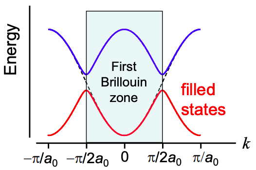
\[ \epsilon =\alpha \pm \sqrt{\beta_{S}^{2}+\beta_{D}^{2}+2\beta_{S}\beta_{D}\ cos\ 2ka_{0}} \nonumber \]

In the alternating bond model, the period of polyacetylene is \(2a_{0}\). Thus the number of distinct k values is \(2\pi /2a_{0}\ /\ 2\pi/L =N/2\), where N is the number of carbon atoms in the polymer backbone.

But there are two solutions for the energy at each k value (i.e. there are two energy bands), so the total number of states is N. Since each state holds two electrons, we find that the bottom band is completely full and the top band is completely empty. Thus, the periodic potential formed by alternating single and double bonds opens a band gap at \(k=\pi/2a_{0}\), completing transforming the material from a metal to an insulator/semiconductor! Obviously, the accuracy of the DOS calculation is critical.

Figure \(\PageIndex{2}\): A periodic perturbation with twice the interatomic spacing introduces a gap at the Fermi energy, transforming a metal into an insulator (wide bandgap semiconductor).

Graphene

Like polyacetylene in the alternating bond model, in graphene we have a unit cell with two carbon atoms. Let the wavefunction of the unit cell be

\[ \phi = c_{1}\phi_{1}+c_{2}\phi_{2} \nonumber \]

where \(\phi_{1}\) and \(\phi_{2}\) are the frontier atomic orbitals of the first and second carbon atom in the unit cell, respectively.

We assume a wavefunction of the Bloch form (Equation (6.18.1)) but we re-write it in terms of a sum over all lattice vectors R:

\[ \psi{\bf{(x) = \sum_{R}e^{ik\cdot R}\phi(x-R)}} . \nonumber \]

Next we define the hopping integral

\[ \beta = \left< \phi_{1}|H|\phi_{2} \right> \nonumber \]

As before, \(\alpha = \left< \phi_{j}|H|\phi_{j} \right>\).

Let's now consider two overlap equations

\[ \left< \phi_{1}({\bf{R}})|H| \psi({\bf{x}})\right> = \epsilon \left< \phi_{1}({\bf{R}})| \psi({\bf{x}})\right> \\
\left< \phi_{2}({\bf{R}})|H| \psi({\bf{x}})\right> = \epsilon \left< \phi_{2}({\bf{R}})| \psi({\bf{x}})\right> . \nonumber \]

Under the Hückel/tight binding approximations, the LHS of Equation (6.18.19)expands to

\[ \left< \phi_{1}({\bf{R}})|H| \psi({\bf{x}})\right> = \left( c_{1}\alpha+c_{2}\beta\left( 1+e^{-ik \cdot \tilde{a_{1}}}+e^{-ik \cdot \tilde{a_{2}}} \right) \right)e^{ik \cdot R} \\
\left< \phi_{2}({\bf{R}})|H| \psi({\bf{x}})\right> = \left( c_{2}\alpha+c_{1}\beta\left( 1+e^{-ik \cdot \tilde{a_{1}}}+e^{-ik \cdot \tilde{a_{2}}} \right) \right)e^{ik \cdot R} \nonumber \]

The RHS of Equation (6.18.19) expands to

\[ \epsilon \left< \phi_{1}({\bf{R}})| \psi({\bf{x}})\right> = \epsilon c_{1}e^{ik \cdot R} \\
\epsilon \left< \phi_{2}({\bf{R}})| \psi({\bf{x}})\right> = \epsilon c_{2}e^{ik \cdot R} \nonumber \]

The solution for non-trivial \(c_{1},\ c_{2}\) is given by

\[ \left|\begin{array}{cc}
\alpha-\varepsilon & \beta\left(1+e^{-i k \cdot \tilde{a}_{1}}+e^{-i k \cdot \tilde{a}_{2}}\right) \\
\beta\left(1+e^{i k \cdot \tilde{a}_{1}}+e^{i k \cdot \tilde{a}_{2}}\right) & \alpha-\varepsilon
\end{array}\right|=0 \nonumber \]

i.e.

\[ \epsilon = \alpha \pm \beta \sqrt{3+2cos({\bf{k \cdot \tilde{a_{1}}}}) +2cos({\bf{k \cdot \tilde{a_{2}}}})+ 2cos({\bf{k \cdot (\tilde{a_{1}}}-\tilde{a_{2}}})} \nonumber \]

This is plotted in Figure 6.18.3, where we have arbitrarily set \(\alpha= 0\).

Figure \(\PageIndex{3}\): The bandstructure of graphene

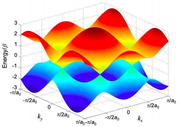
Each unit cell contributes an orbital to a band; given N unit cells, each band has N states, or including spin, 2N states. Graphene, with two electrons per unit cell has two bands and 2N electrons. Thus, the lower band of graphene is completely filled.

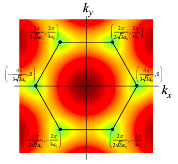
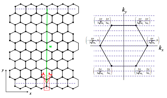
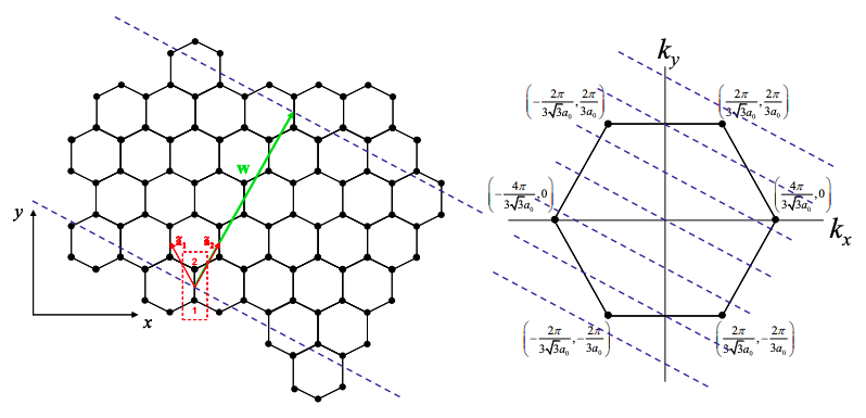
We might therefore expect that graphene is an insulator, but the lower band touches the upper band at values of k known as the K points

\[ {\bf{K}} = \left( \pm \frac{4\pi}{3\sqrt{3a_{0}}},0 \right),\ \left( \pm \frac{2\pi}{3\sqrt{3a_{0}}}, \pm \frac{2\pi}{3a_{0}} \right) \nonumber \]

Thus, in these particular directions graphene conducts like a metal.

Figure \(\PageIndex{4}\): The K points in graphene.

Carbon Nanotubes

Carbon nanotubes are remarkable materials. They are perhaps the most rigid materials known, and they have excellent charge transport properties.

Figure \(\PageIndex{5}\): An example of a carbon nanotube – composed of a rolled up graphene sheet. This particular tube is known as an armchair – you may be able to identify armchairs in the hexagonal lattice.

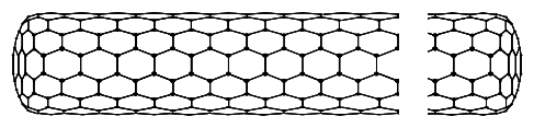
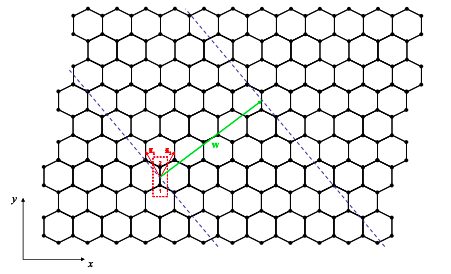
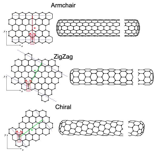
We will treat carbon nanotubes as rolled-up graphene sheets. The construction of a nanotube from a sheet of graphene can be imagined as in Figure 6.18.6. We first draw the wrapping vector from one unit cell to another. When the tube is formed both ends of the wrapping vector will be connected. The wrapping vector is written

\[ {\bf{w}}=n{\bf{\tilde{a_{1}}}}+m{\bf{\tilde{a_{2}}}} = (n,m) \nonumber \]

The length of the wrapping vector determines the circumference of the tube, and as we shall see the vector (n,m) characterizes its electronic properties.

Next two parallel cuts are made perpendicular to the wrapping vector and the remaining piece is rolled up; see Figure 6.18.7.\(^{†}\)

Figure \(\PageIndex{6}\): . Carbon nanotubes can be imagined to be constructed from rolled up pieces of graphene. In the example above, a wrapping vector, w, is drawn between two unit cells that will be connected when the tube is rolled up. The graphene sheet is cut perpendicular to w.

After the tube is rolled up, periodic boundary conditions are established on the circumference of the tube. Thus, only certain values of the wavevector, k, are allowed perpendicular to the tube axis, i.e.

\[ {\bf{k \cdot w}}= 2\pi l,\ l \in \mathbb{Z} \nonumber \]

If the allowed k-states include the K points of graphene then the carbon nanotube will be a metal, otherwise it is a semiconductor. For example, consider a (4,4) armchair nanotube as shown below. We also plot the K points for graphene in k space.

Figure \(\PageIndex{7}\): Three types of nanotubes. The first two, armchair and zigzag are special cases with wrapping vectors (N,N) and (N,0) or (0,N), respectively. The third is the general case or chiral form with wrapping vector (n,m).

Figure \(\PageIndex{8}\): At left, a (4,4) armchair nanotube. At right, the K points of graphene.

Let‟s begin by decomposing k into a component perpendicular to the tube axis, \({\bf{k_{\perp}}}\), and a component parallel to the tube axis, \({\bf{k_{\parallel}}}\). For a (4,4) tube \({\bf{w}} = 12a_{0}{\bf{\hat{y}}}\). Thus, the allowed values of k are given by

\[ k_{y}=\frac{\pi l}{6a_{0}} . \nonumber \]

As shown in Fig. 6.18.8, this set of allowed \({\bf{k_{\perp}}}\) values includes the K points. Thus (4,4) tubes are metallic.

Next, let's examine a (0,4) zigzag tube.

Figure \(\PageIndex{9}\): At left, a (0,4) zigzag nanotube. At right, the K points of graphene.

For a (0,4) tube \({\bf{w}} = 2\sqrt{3}a_{0}{\bf{\hat{x}}}+6a_{0}{\bf{\hat{y}}}\). Thus, the allowed values of \({\bf{k_{\perp}}}\) are given by

\[ 2\sqrt{3}k_{x}+6k_{y} = \frac{2\pi l}{a_{0}} . \nonumber \]

As shown in Figure 6.18.9, this set of allowed k values does not include the K points. Thus (0,4) tubes are insulating/semiconducting.

\(^{†}\)Of course, carbon nanotubes are not actually made from graphene like this. There are many techniques including chemical vapor deposition using a catalyst particle that defines the width of the tube.