6.20: Analytic approximations for the bandstructure of graphene and carbon nanotubes
- Page ID
- 52375
Since the conduction properties of graphene are dominated by electrons occupying states at or near the K points, it is convenient to linearize the energy at \({\bf{\kappa = k+K}}\).
The exact tight binding solution from Equation (6.18.23) is:
\[ \varepsilon = \alpha \pm \beta \sqrt{3+ 2cos({\bf{k\cdot\tilde{a_{1}}}})+2cos({\bf{k\cdot\tilde{a_{2}}}})+2cos({\bf{k\cdot(\tilde{a_{1}}-\tilde{a_{2}})}})} \nonumber \]
We substitute \(\bf{k = K+\kappa}\) and expand the \(cos({\bf{K+\kappa}})\) terms as a Taylor series to second order in \(\kappa\). This yields:
\[ \varepsilon = \alpha \pm \beta \sqrt{3 +2cos({\bf{K\cdot\tilde{a_{1}}}})+2cos({\bf{K\cdot\tilde{a_{2}}}})+2cos({\bf{K\cdot(\tilde{a_{1}}-\tilde{a_{2}}}}))+2{\bf{\kappa \cdot \tilde{a_{1}}}}sin({\bf{K\cdot \tilde{a_{1}}}})+2{\bf{\kappa \cdot \tilde{a_{2}}}}sin({\bf{K\cdot \tilde{a_{2}}}})+2{\bf{\kappa \cdot (\tilde{a_{1}}}-\tilde{a_{2}})}sin({\bf{K\cdot (\tilde{a_{1}}}-\tilde{a_{2}})})-({\bf{\kappa \cdot \tilde{a_{1}}}})^{2}cos({\bf{K\cdot\tilde{a_{1}}}})-({\bf{\kappa \cdot \tilde{a_{2}}}})^{2}cos({\bf{K\cdot\tilde{a_{2}}}})-({\bf{\kappa \cdot (\tilde{a_{1}}-\tilde{a_{2}})}})^{2}cos({\bf{K\cdot(\tilde{a_{1}}-\tilde{a_{2}})}})} \nonumber \]
Next, we note some identities:
\[ cos({\bf{K\cdot\tilde{a_{1}}}}) = cos({\bf{K\cdot\tilde{a_{2}}}}) = cos({\bf{K\cdot(\tilde{a_{1}}-\tilde{a_{2}})}}) = -\frac{1}{2} \nonumber \]
\[ sin({\bf{K\cdot\tilde{a_{1}}}}) = -sin({\bf{K\cdot\tilde{a_{2}}}}) = -sin({\bf{K\cdot(\tilde{a_{1}}-\tilde{a_{2}})}}) \nonumber \]
From these identities Equation (6.19.2) reduces to
\[ \varepsilon = \alpha \pm \beta \sqrt{\frac{1}{2}({\bf{\kappa \cdot \tilde{a_{1}}}})^{2}+\frac{1}{2}({\bf{\kappa \cdot \tilde{a_{2}}}})^{2}+\frac{1}{2}({\bf{\kappa \cdot (\tilde{a_{1}}}-\tilde{a_{2}})})^{2}} \nonumber \]
Solving this (see the Problem Set) gives the approximate dispersion relation for graphene:
\[ \varepsilon = \alpha \pm \frac{3}{2}\beta |\kappa| \nonumber \]
Since the speed of the charge carrier is given by the group velocity: \(v = \hbar^{-1} \partial \varepsilon/\partial k\), we get
\[ v = \frac{3}{2}\frac{\beta a_{0}}{\hbar} \nonumber \]
For \(a_{0} = 1.42\AA\) and \(\beta = 2.5\ eV\), \(v = 10^{6}\ m/s\)
Now, for carbon nanotubes, the periodic boundary condition on the circumfrence is
\[ {\bf{\kappa + K}\cdot w} = 2\pi l, l \in \mathbb{Z} \nonumber \]
Let's consider each K point in turn:
For \({\bf{K}}= \left( \frac{4\pi}{3\sqrt{3}a_{0}}, 0 \right)\)
\[ {\bf{(\kappa + K})\cdot w} = {\bf{\kappa \cdot w + K \cdot}}(n {\bf{\tilde{a_{1}}}}+m{\bf{\tilde{a_{2}}}}) \\
= {\bf{\kappa \cdot w}} + n{\bf{K \cdot}} \left( -\frac{\sqrt{3}}{2}a_{0}, \frac{3}{2}a_{0} \right)+m{\bf{K \cdot}} \left( \frac{\sqrt{3}}{2}a_{0}, \frac{3}{2}a_{0} \right) \\
= {\bf{\kappa \cdot w}} + \frac{2\pi}{3} (m-n) \nonumber \]
Rearranging gives:
\[ {\bf{\kappa \cdot w}} = 2\pi l + 2\pi \frac{(n-m)}{3} \nonumber \]
For \({\bf{K}}= \left( \frac{2\pi}{3\sqrt{3}a_{0}}, \frac{2\pi}{3a_{0}} \right)\)
\[ {\bf{\kappa \cdot w}}= 2\pi l + 2\pi \frac{(2n+m)}{3} \\
=2\pi l + 2\pi \frac{(3n-(n-m))}{3} \\
\equiv 2\pi l - 2\pi \frac{(n-m)}{3} \nonumber \]
For \({\bf{K}}= \left( -\frac{2\pi}{3\sqrt{3}a_{0}}, \frac{2\pi}{3a_{0}} \right)\)
\[ {\bf{\kappa \cdot w}}= 2\pi l + 2\pi \frac{(n+2m)}{3} \\
=2\pi l + 2\pi \frac{((n-m)+3m))}{3} \\
\equiv 2\pi l + 2\pi \frac{(n-m)}{3} \nonumber \]
The other K points follow by symmetry, and we can conclude that
\[ {\bf{\kappa}}_{\perp} = \frac{2\pi}{|{\bf{w}}|} \left( l + \frac{(n-m)}{3} \right) \nonumber \]
where we have separated \(\kappa\) into two components parallel, \(\kappa_{\parallel}\), and perpendicular, \kappa_{\perp} to the tube axis. From Equation (6.19.6) we get
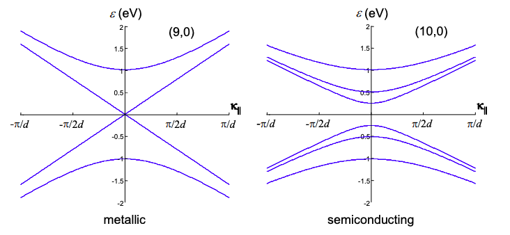
\[ \varepsilon = \alpha \pm \frac{3\beta a_{0}}{d} \sqrt{\left( l + \left( \frac{n-m}{3} \right) \right)^{2}+ \left( \frac{\kappa_{\parallel}d}{2} \right)^{2}} . \nonumber \]
where the tube circumference is \(|{\bf{w}}| = \pi d\). Interestingly, Eq. (6.98) predicts that tubes are metallic when \([(n-m)/3] \in \mathbb{Z}\). Assuming that n and m are generated randomly, we expect that 1/3 of tubes should be metallic. Indeed, this seems to be the case in practice. Note also that for semiconducting tubes the band gap is inversely proportional to the tube diameter.