Engineering LibreTexts

6.17: Odds and Ends

  • Page ID
    88589
  • \( \newcommand{\vecs}[1]{\overset { \scriptstyle \rightharpoonup} {\mathbf{#1}} } \) \( \newcommand{\vecd}[1]{\overset{-\!-\!\rightharpoonup}{\vphantom{a}\smash {#1}}} \)\(\newcommand{\id}{\mathrm{id}}\) \( \newcommand{\Span}{\mathrm{span}}\) \( \newcommand{\kernel}{\mathrm{null}\,}\) \( \newcommand{\range}{\mathrm{range}\,}\) \( \newcommand{\RealPart}{\mathrm{Re}}\) \( \newcommand{\ImaginaryPart}{\mathrm{Im}}\) \( \newcommand{\Argument}{\mathrm{Arg}}\) \( \newcommand{\norm}[1]{\| #1 \|}\) \( \newcommand{\inner}[2]{\langle #1, #2 \rangle}\) \( \newcommand{\Span}{\mathrm{span}}\) \(\newcommand{\id}{\mathrm{id}}\) \( \newcommand{\Span}{\mathrm{span}}\) \( \newcommand{\kernel}{\mathrm{null}\,}\) \( \newcommand{\range}{\mathrm{range}\,}\) \( \newcommand{\RealPart}{\mathrm{Re}}\) \( \newcommand{\ImaginaryPart}{\mathrm{Im}}\) \( \newcommand{\Argument}{\mathrm{Arg}}\) \( \newcommand{\norm}[1]{\| #1 \|}\) \( \newcommand{\inner}[2]{\langle #1, #2 \rangle}\) \( \newcommand{\Span}{\mathrm{span}}\)\(\newcommand{\AA}{\unicode[.8,0]{x212B}}\)

    Just a few odds and ends. Consider Figure \(\PageIndex{1}\), which is called a "cascaded line" problem. These are problems where we have two different transmission lines, with different characteristic impedances. Since we will give all of the distances in wavelengths, λ, we will assume that the λ we are talking about is the appropriate one for the line involved. If the phase velocities on the two lines is the same, then the physical lengths would correspond as well. The approach is relatively straight-forward. First let's plot Z L Z 0 Z L Z 0 on the Smith Chart, in Figure \(\PageIndex{2}\). Then we have to rotate 0.2λ 0.2 λ so that we can find Z A Z 0 1 Z A Z 0 1 , the normalized impedance at point A, the junction between the two lines in Figure \(\PageIndex{3}\).

    A transmission line with a 50-Ohm impedance Z_02 and length 0.15 lambda transitions into a second transmission line with a 300-Ohm impedance Z_01 and length 0.2 lambda at point A. The right end of this transmission line connects to a load impedance of the sum 2 + 2j, times Z_01.

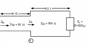
    Figure \(\PageIndex{1}\): Cascaded line

    Smith Chart containing the point representing Z_L/Z_01, with a real component of 2 and an imaginary component of 2j.

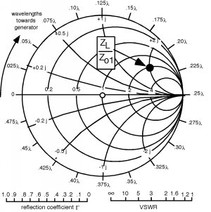
    Figure \(\PageIndex{2}\): Smith Diagram

    Thus, we find Z A Z 0 1 =0.32+0.6i Z A Z 0 1 0.320.6 . Now we have to renormalize the impedance so we can move to the line with the new impedance Z 0 2 Z 0 2 . Since Z 0 1 =300Ω Z 0 1 300 Ω , Z A =96+-180i Z A 96-180 . This is the load for the second length of line, so let's find Z A Z 0 2 Z A Z 0 2 , which is easily found to be 1.9+-3.6i 1.9-3.6, so this can be plotted on the Smith Chart in Figure \(\PageIndex{4}\). Now we have to rotate around another 0.15λ 0.15 λ so that we can find Z in Z 0 2 Z in Z 0 2 . This appear to have a value of about 0.15+-0.45i 0.15-0.45, so Z in =7.5+-22.5iΩ Z in 7.5-22.5 Ω, as shown in Figure \(\PageIndex{5}\).

    Rotating clockwise about the Smith Chart on a circle of constant radius by a distance of 0.2 lambda, from the point representing Z_L/Z_01 to the point representing Z_A/Z_01.

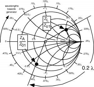
    Figure \(\PageIndex{3}\): Towards the generator

    Smith Chart labeled with the three points representing Z_L/Z_01, Z_A/Z_01, and Z_A/Z_02.

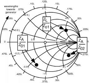
    Figure \(\PageIndex{4}\): More Smith Charts

    Moving clockwise on the Smith Chart by a distance of 0.15 lambda, from the point representing Z_A/Z_02 along a circle of constant radius to the point representing Z_in/Z_02.

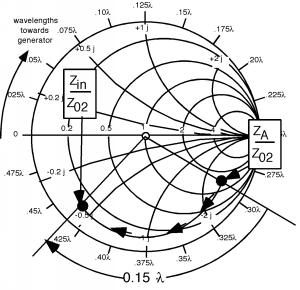
    Figure \(\PageIndex{5}\): Even more Smith Charts

    There is one application of the cascaded line problem that is used quite a bit in practice. Consider the following: We assume that we have a matched line with impedance Z 0 2 Z 0 2 and we connect it to another line whose impedance is Z 0 1 Z 0 1  as shown in Figure \(\PageIndex{6}\). If we connect the two of them together directly, we will have a reflection coefficient at the junction given by

    Γ= Z 0 2 Z 0 1 Z 0 2 + Z 0 1 Γ Z 0 2 Z 0 1 Z 0 2 Z 0 1
    Simplified cascaded line, with a line of impedance Z_01 on the left leading into a line of  impedance Z_02 on the right.

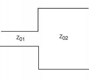
    Figure \(\PageIndex{6}\): Simplified cascaded line

    Now let's imagine that we have inserted a section of line with length l=λ4 l λ 4 and impedance Z m Z m  as in Figure \(\PageIndex{7}\). At point \(A\), the junction between the first line and the matching section, we can find the normalized impedance as

    Z A Z M = Z 0 2 Z m Z A Z M Z 0 2 Z m
    At point B, a cascade line with impedance Z_01 leads into a line of impedance Z_M and length lambda/4. At point A, the line with impedance Z_M leads into another line with impedance Z_02.

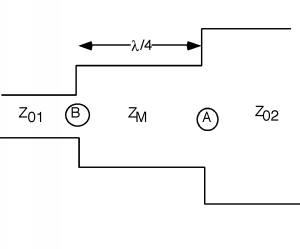
    Figure \(\PageIndex{7}\): Another cascaded line

    We take this impedence and rotate around on the Smith Chart λ4 λ 4 to find Z B Z M Z B Z M

    Z B Z M = Z m Z 0 2 Z m Z B Z M Z m Z 0 2 Z m

    where we have taken advantage of the fact that when we go half way around the Smith Chart, the impedance we get is just the inverse of what we had originally (half way around turns rs r s into rs r s ).

    Thus

    Z B = Z m 2 Z 0 2 Z B Z m 2 Z 0 2

    If we want to have a match for line with impedence Z 0 1 Z 0 1 , then Z B Z B should equal Z 0 1 Z 0 1 and hence:

    Z B = Z 0 1 = Z m 2 Z 0 2 Z B Z 0 1 Z m 2 Z 0 2

    or

    Z m = Z 0 1 Z 0 2 Z m Z 0 1 Z 0 2

    This piece of line is called a quarter wave matching section and is a convenient way to connect two lines of different impedance.


    This page titled 6.17: Odds and Ends is shared under a CC BY 1.0 license and was authored, remixed, and/or curated by Bill Wilson via source content that was edited to the style and standards of the LibreTexts platform; a detailed edit history is available upon request.

    • Was this article helpful?