2.8: Return Loss, Substitution Loss, and Insertion Loss

2.8.1 Return Loss

Return loss, also known as reflection loss, is a measure of the fraction of power that is not delivered by a source to a load. If the power incident on a load is \(P_{i}\) and the power reflected by the load is \(P_{r}\), then the return loss in decibels is [6, 7]

\[\label{eq:1}\text{RL}_{\text{dB}}=10\log\frac{P_{i}}{P_{r}} \]

The better the load is matched to the source, the lower the reflected power and hence the higher the return loss. \(\text{RL}\) is a positive quantity if the reflected power is less than the incident power. If the load has a complex reflection coefficient \(\rho\), then

\[\label{eq:2}\text{RL}_{\text{dB}}=10\log\left|\frac{1}{\rho^{2}}\right|=-20\log|\rho| \]

That is, the return loss is the negative of the input reflection coefficient expressed in decibels [8].

When generalized to a terminated two ports, the return loss is defined with respect to the input reflection coefficient of the terminated two port [9]. The two port in Figure \(\PageIndex{1}\) has the input reflection coefficient

\[\label{eq:3}\Gamma_{\text{in}}=S_{11}+\frac{\Gamma_{L}S_{12}S_{21}}{(1-\Gamma_{L}S_{22})} \]

where \(\Gamma_{L}\) is the reflection coefficient of the load. Thus the return loss of a terminated two-port is

\[\label{eq:4}\text{RL}_{\text{dB}}=-20\log|\Gamma_{\text{in}}|=-20\log\left|S_{11}+\frac{\Gamma_{L}S_{12}S_{21}}{(1-\Gamma_{L}S_{22})}\right| \]

If the load is matched, i.e. \(Z_{L} = Z_{0}^{\ast}\) (the system reference impedance), then

\[\label{eq:5}\text{RL}_{\text{dB}}=-20\log|S_{11}| \]

This return loss is also called the input return loss since the reflection coefficient is calculated at Port \(\mathsf{1}\). The output return loss is calculated looking into Port \(\mathsf{2}\) of the two-port, where now the termination at Port \(\mathsf{1}\) is just the source impedance.

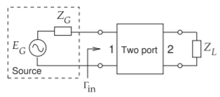
Figure \(\PageIndex{1}\): Terminated two-port used to define return loss.

2.8.2 Substitution Loss and Insertion Loss

The substitution loss is the ratio of the power, \(^{i}P_{L}\), delivered to the load by an initial two-port identified by the leading superscript ‘\(i\)’, and the power delivered to the load, \(^{f}P_{L}\), with a substituted final two-port identified by the leading superscript ‘\(f\)’. In terms of generalized scattering parameters with reference impedances \(Z_{01}\) at Port \(\mathsf{1}\) and \(Z_{02}\) at Port \(\mathsf{2}\) the substitution loss in decibels is (using the results of Example 3.2.2 and noting that \(\Gamma_{S}\) is referred to \(Z_{01}\) and \(\Gamma_{L}\) is referred to \(Z_{02}\))

\[\label{eq:6}L_{S}|_{\text{dB}}=\frac{^{i}P_{L}}{^{f}P_{L}}=10\log\left|\frac{^{i}P_{L}}{^{f}P_{L}}\frac{[(1 −\:^{f}S_{11}\Gamma_{S})(1 −\:^{f}S_{22}\Gamma_{L}) −\:^{f}S_{12}\:^{f} S_{21}\Gamma_{S}\Gamma_{L}]}{[(1 −\:^{i}S_{11}\Gamma_{S})(1 −\:^{i}S_{22}\Gamma_{L}) −\:^{i}S_{12}\:^{i}S_{21}\Gamma_{S}\Gamma_{L}]}\right|^{2} \]

Insertion loss is a special case of substitution loss with particular types of initial two-port networks. There are a number of special cases to consider.

Insertion Loss with an Ideal Adaptor

Comparing the power delivered to the load with an inserted two-port with that delivered with an ideal adaptor is the commonly accepted definition of insertion loss [10]. That is, ‘insertion loss’ without qualifications is the same as ‘insertion loss with an ideal adaptor.’ An ideal adaptor (as the initial two-port network) transforms from the Port \(\mathsf{1}\) reference impedance, \(Z_{01}\), to the Port \(\mathsf{2}\) reference impedance, \(Z_{02}\). In terms of generalized \(S\) parameters the ideal adaptor has \(^{i}(\:^{G}S_{11}) =0=\:^{i}(\:^{G}S_{22})\) (for no reflection), \(^{i}(^{G}S_{12})\:^{i}(\:^{G}S_{21}) = 1\) (for no loss in the adaptor and there is no phase shift), and \(^{i}(\:^{G}S_{12}) =\:^{i}(\:^{G}S_{21}) Z_{01}/Z_{02}\) (for reciprocity). (If \(Z_{01} = Z_{02}\) this ideal adaptor is the same as a direct connection.) Insertion loss in decibels is, using Equation \(\eqref{eq:6}\):

\[\label{eq:7}\text{IL}|_{\text{dB}}=10\log\left\{\frac{Z_{02}}{Z_{01}}\left|\frac{[1 −\:^{f}(\:^{G}S_{11})\Gamma_{S}]\:[1 −\:^{f}(\:^{G}S_{22})\Gamma_{L}] −\:^{f}(\:^{G}S_{12})\:^{f}(\:^{G}S_{21})\Gamma_{S}\Gamma_{L}}{^{f}(\:^{G}S_{12})(1-\Gamma_{S}\Gamma)}\right|^{2}\right\} \]

Attenuation is defined as the insertion loss without source and load reflections \((\Gamma_{S} =0=\Gamma_{L})\) [10], and Equation \(\eqref{eq:7}\) becomes

\[\label{eq:8}A|_{\text{dB}}=10\log\left(\frac{Z_{02}}{Z_{01}}\frac{1}{|^{G}S_{21}|^{2}}\right)\quad (=\text{IL}|_{\text{dB}}\text{ with }\Gamma_{S}=0=\Gamma_{L}) \]

where \(^{G}S_{21}\) is that of the final two-port.

Insertion Loss with Direct Connection

With normalized \(S\) parameters, i.e. \(Z_{01} = Z_{02}\), the insertion loss with an initial direct connection is as given in Equation \(\eqref{eq:7}\). With different reference impedances at each port, the initial direct connection ‘\(i\)’, from Example 2.4.1, \(^{i}(\:^{G}S_{11})= (Z_{02} − Z_{01})/(Z_{02} + Z_{01}),\) \(^{i}(\:^{G}S_{22}) = −\:^{i}(\:^{G}S_{11}),\) \(^{i}(\:^{G}S_{21}) = [1 +\:^{i}(\:^{G}S_{11})]\times\sqrt{\Re \{Z_{02}\}}/\sqrt{\Re \{Z_{01}\}}\), and \(^{i}(\:^{G}S_{12}) =[1 +\:^{i}(\:^{G}S_{22})]\sqrt{\Re\{Z_{01}\}}/ \sqrt{\Re\{Z_{02}\}}\). These \(S\) parameters of the initial two-port network are substituted in Equation \(\eqref{eq:6}\) to determine insertion loss with a direct connection.

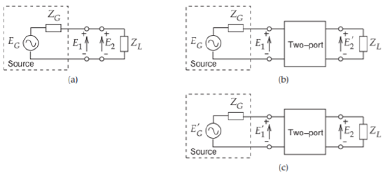
Figure \(\PageIndex{2}\): Two-port insertion and definition of variables for defining insertion loss: (a) source and load before insertion; (b) insertion of two-port network with source level unchanged; and (c) insertion of two-port network with source level adjusted to maintain a constant voltage across the load.

2.8.3 Measurement of Insertion Loss

If the \(S\) parameters of a two-port network can be measured it is simple to calculate the insertion loss of the two-port. However there are situations where the \(S\) parameters cannot be measured and this includes where there is not a port connection (e.g., the air side of an antenna) and the system reference impedances differ at the two ports. In this section methods for measuring insertion loss in such difficult situations is described. If \(S\) parameter measurements are not available the insertion loss of a two-port network is defined as the ratio, in decibels, of voltages immediately beyond the point of insertion, before and after insertion [6, 11]. Referring to Figure \(\PageIndex{2}\)(a and b), insertion loss is expressed in decibels as

\[\label{eq:9}\text{IL}_{\text{dB}}=20\log\left|\frac{E_{2}}{E_{2}'}\right| \]

where \(E_{2}\) is the voltage across the load \((Z_{L})\) before insertion of the two-port and \(E_{2}′\) is the voltage across the load \((Z_{L})\) after insertion of the two-port. The power delivered to the load is proportional to the square of the magnitude of the voltage across the load, so this definition is equivalent to that described in section 2.8.2 where

\[\label{eq:10}\text{IL}_{\text{dB}}=10\log\frac{P_{L}}{P_{T}} \]

where \(P_{L}\) is the power delivered to the load before the insertion of the two-port and \(P_{T}\) is the power delivered to the load following insertion.

Example \(\PageIndex{1}\): Insertion loss of a two-port in a different reference system

A \(50\:\Omega\) attenuator has an attenuation of \(3\text{ dB}\) and a return loss of \(20\text{ dB}\). If the attenuator is used in a \(75\:\Omega\) system what is the insertion loss of the attenuator?

Solution

The insertion loss can be calculated using the insertion loss formula in Equation \(\eqref{eq:6}\). To apply this the \(50\:\Omega\text{ S}\) parameters of the attenuator are needed and then the load and source reflection coefficients, \(\Gamma_{L}\) and \(\Gamma_{S}\) respectively, which will be the reflection coefficients of the \(75\:\Omega\) load and source impedances referred to \(50\:\Omega\). Also note that \(Z_{01} = Z_{02} = 50\:\Omega\). Since there are two reference systems the leading superscripts \(50\) and \(75\) will be used to distinguish them.

\(\underline{\text{Step 1.}}\) Find \(\Gamma_{S}\) and \(\Gamma_{L}\) in the \(50\:\Omega\) system: \(\Gamma_{S} =\Gamma_{L} = (55 − 50)/(55 + 50) = 0.2000\)

\(\underline{\text{Step 2.}}\) Find the \(S\) parameters in a \(50\:\Omega\) system. (case \(\mathsf{1}\), assume \(\angle S_{11} =\angle S_{21} = 0^{\circ})\)

It is known that \(^{50}\text{RL}|_{\text{dB}} = 20\text{ dB}\) and \(^{50}\text{IL}|_{\text{dB}} = 3\text{ dB}\). Also an attenuator is symmetrical so that \(^{50}S_{11} =\:^{50}S_{22}\) and \(^{50}S_{12} =\:^{50}S_{21}\). Using Equations \(\eqref{eq:5}\) and \(\eqref{eq:8}\)

\[|^{50}S_{11}|=|^{50}S_{22}|=10^{-50_{\text{RL}|_{\text{dB}}/20}}=10^{-20/20}=0.1000\nonumber \]

and

\[|^{50}S_{12}|=|^{50}S_{21}|=10^{-50_{\text{IL}|_{\text{dB}}/20}}=10^{-3/20}=0.7080\nonumber \]

The phases of the \(S\) parameters are not known. Assume first (use the leading subscript ‘\(1\)’) that the phases are \(0^{\circ}\) and consider alternatives later and then the \(S\) parameter matrix is

\[\label{eq:11}_{1}\mathbf{S}=\left[\begin{array}{cc}{^{50}_{1}S_{11}}&{^{50}_{1}S_{12}}\\{^{50}_{1}S_{21}}&{^{50}_{1}S_{22}}\end{array}\right]=\left[\begin{array}{cc}{0.1000}&{0.7080}\\{0.7080}&{0.1000}\end{array}\right] \]

From Equation \(\eqref{eq:7}\)

\[\label{eq:12}^{75}_{1}\text{IL}_{\text{dB}}=10\log\left[\frac{50}{50}\left|\frac{(1 − 0.1\cdot 0.2) (1 − 0.1\cdot 0.2) − 0.7080\cdot 0.7080\cdot 0.2\cdot 0.2}{0.7080 (1 − 0.2\cdot 0.2)}\right|^{2}\right]=2.82\text{ dB} \]

\(\underline{\text{Step 3}}\) Four phase assumptions for \(S_{11}\) and \(S_{22}\)

\[\begin{array}{lll}{\text{Case 1}}&{\angle S_{11}=\angle S_{22}=0^{\circ},\:\angle S_{21}=\angle S_{12}=0^{\circ}}&{^{75}_{1}\text{IL}_{\text{dB}}=2.82\text{ dB}}\\{\text{Case 2}}&{\angle S_{11}=\angle S_{22}=0^{\circ},\:\angle S_{21}=\angle S_{12}=180^{\circ}}&{^{75}_{2}\text{IL}_{\text{dB}}=2.82\text{ dB}}\\{\text{Case 3}}&{\angle S_{11}=\angle S_{22}=180^{\circ},\:\angle S_{21}=\angle S_{12}=0^{\circ}}&{^{75}_{3}\text{IL}_{\text{dB}}=3.53\text{ dB}}\\{\text{Case 4}}&{\angle S_{11}=\angle S_{22}=180^{\circ},\:\angle S_{21}=\angle S_{12}=180^{\circ}}&{^{75}_{4}\text{IL}_{\text{dB}}=3.53\text{ dB}}\end{array}\nonumber \]

Thus just knowing the return loss and insertion loss in one reference system is not enough to know the insertion loss in another system without knowing the phases of the \(S\) parameters.

Example \(\PageIndex{2}\): Insertion loss calculation using change of reference impedance

A \(50\:\Omega\) attenuator has an attenuation of \(3\text{ dB}\) and a return loss of \(20\text{ dB}\). If the attenuator is use in a \(75\:\Omega\) system what is the insertion loss of the attenuator?

Solution

This is alternative to the method used in Example \(\PageIndex{1}\). Using the \(S\) parameters of the attenuator in Equation \(\eqref{eq:11}\), in a \(75\:\Omega\) system the \(S\) parameters are found using Equation (2.4.30) and noting that \(\Gamma_{75} = 0.2\) is the reflection coefficient of \(75\:\Omega\) in a \(50\:\Omega\) system:

\[\begin{align}^{75}\mathbf{S}&=\left[\begin{array}{cc}{^{75}S_{11}}&{^{75}S_{12}} \\ {^{75}S_{21}}&{^{75}S_{22}}\end{array}\right]=\left[\begin{array}{cc}{^{50}_{1}S_{11}-\Gamma_{75}}&{^{50}_{1}S_{12}}\\{^{50}_{1}S_{21}}&{^{50}_{1}S_{22}-\Gamma_{75}}\end{array}\right]\left[\begin{array}{cc}{1-\Gamma_{75}\:^{50}_{1}S_{11}}&{-\Gamma_{75}\:^{50}_{1}S_{12}}\\{-\Gamma_{75}\:^{50}_{1}S_{21}}&{1-\Gamma_{75}\:^{50}_{1}S_{22}}\end{array}\right]^{-1} \nonumber \\ \label{eq:13}&=\left[\begin{array}{cc}{-0.1}&{0.7080} \\ {0.7080}&{-0.1}\end{array}\right]\left[\begin{array}{cc}{0.9800}&{-0.1416} \\ {-0.1416}&{0.9800}\end{array}\right]^{-1}=\left[\begin{array}{cc}{0.002379}&{0.7227} \\ {0.7227}&{0.002379}\end{array}\right]\end{align} \]

In the \(75\:\Omega\) system the load and source are matched and using Equation \(\eqref{eq:7}\)

\[\label{eq:14}^{75}_{1}\text{IL}_{\text{dB}}=10\log\frac{1}{|^{75}S_{21}|^{2}}=10\log\frac{1}{|0.7227|^{2}}=2.82\text{ dB} \]

which is in agreement with the calculation in Example \(\PageIndex{1}\), see Equation \(\eqref{eq:12}\).

2.8.4 Minimum Transducer Loss, Intrinsic Attenuation

Another situation often required is determining the minimum possible loss of a two-port. This is obtained with lossless two-port networks, \(M_{1}\) and \(M_{2}\) at the input and output of the two-port of interest, \(M_{3}\). \(M_{1}\) and \(M_{2}\) are adjusted to obtained the minimum possible loss of \(M_{3}\). This is not the same as designing \(M_{1}\) and \(M_{2}\) to obtain matching. The minimum insertion loss, also called the intrinsic attenuation, or minimum transducer loss in \(\text{dB}\) is [12] (the derivation is involved),

\[\label{eq:15}L_{\text{TM}|\text{dB}}=10\log\left[\frac{Z_{02}}{Z_{01}}\frac{|1 − S_{22}\Gamma_{\text{TM}}|^{2} − |(S_{12}S_{21} − S_{11}S_{22})\Gamma_{\text{TM}} + S_{11}| ^{2}}{|S_{21}|^{2} (1 − |\Gamma_{\text{TM}}|^{2})}\right] \]

where the \(S\) parameters are of \(M_{3}\) \(Z_{01}\) and \(Z_{02}\) are the real reference impedances at ports \(\mathsf{1}\) and \(\mathsf{2}\) respectively, and

\[\label{eq:16}\Gamma_{\text{TM}}=\frac{B}{2A}\left(1\pm\sqrt{1-\frac{2|A|}{B}}\right) \]

where

\[\label{eq:17}A = S_{22} + S_{11}^{\ast} (S_{12}S_{21} − S_{11}S_{22}) \]

and

\[\label{eq:18}B = 1 − |S_{11}|^{2} + |S_{22}|^{2} − |S_{12}S_{21} − S_{11}S_{22}|^{2} \]

The intrinsic attenuation is a useful metric when a device is being developed and has not yet been optimally matched.

Other insertion loss concepts are comparison loss, mismatch loss, and conjugate mismatch loss, see [10].