3.5: Transmission Lines and Smith Charts

The locus of a transmission line on a Smith chart is a circle. When the characteristic impedance of the line is equal to the system reference impedance this circle is centered at the origin of the Smith chart. The main purpose of this section is to consider the situation where the characteristic impedance and the system reference impedance differ.

3.5.1 Bilinear Transform

Mathematically the input reflection coefficient of a terminated transmission line of characteristic impedance \(Z_{02}\) is referenced to a system impedance \(Z_{01}\). The mathematics describing this is based on the bilinear transform. The generalized bilinear transform of two complex numbers \(z\) and \(w\) is

\[\label{eq:1}w=\frac{Az+B}{Cz+D} \]

where \(A,\: B,\: C,\) and \(D\) are constants\(^{1}\) that may themselves be complex. This is of interest in dealing with reflection coefficients where \(w\) and \(z\) are reflection coefficients and \(A,\: B,\: C,\) and \(D\) describe the two-port network connected to a load with a complex reflection coefficient \(z\), and \(w\) is the reflection coefficient looking into the network. The special property of the bilinear transform is that a circle in the complex plane (here the locus of \(z\)) is mapped onto another circle (here the locus of \(w\)) in the complex plane. (This is shown in Section 1.A.14 of [11].)

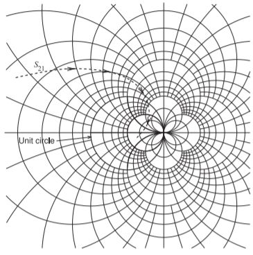
Figure \(\PageIndex{1}\): Expanded Smith chart used to plot scattering parameters with a magnitude greater than \(1\). The forward transmission parameter, \(S_{21}\), of a transistor is shown with the arrows in the direction of increasing frequency. The unit circle of a conventional Smith chart is shown.

3.5.2 Reference Impedance Change as a Bilinear Transform

In Figure \(\PageIndex{2}\) a fixed load terminates a transmission line of characteristic impedance \(Z_{01}\) and the input reflection coefficient is \(\Gamma_{\text{in}}\). As will be shown, the locus of \(\Gamma_{\text{in}}\), normalized to any system impedance, is a circle on the complex plane as the electrical length of the line increases. The electrical length of the line increases as the frequency increases with the physical length of the line held constant, or as the physical length of the line increases with the frequency held constant.

From Equation ((2.3.4)) of [11] the reflection coefficient of a load \(Z_{L}\) referenced to \(Z_{01}\) is

\[\label{eq:2}\Gamma_{L, Z01}=\frac{Z_{L}-Z_{01}}{Z_{L}+Z_{01}} \]

and the input reflection coefficient referenced to \(Z_{01}\) is

\[\label{eq:3}\Gamma_{\text{in }, Z01}=\Gamma_{L, Z01}\text{e}^{-\jmath 2\theta} \]

where \(\theta = \beta\ell\) is the electrical length of the line. As \(\theta\) increases from zero, \(\Gamma_{\text{in, }Z01}\) plotted on a polar chart traces out a circle rotating in the clockwise direction. The important result that will be developed in this section is that when the input reflection coefficient is referenced to another impedance, the new reflection coefficient will also trace out a circle. The development of \(\Gamma_{\text{in, }Z02}\) (the input reflection coefficient referred to \(Z_{02}\)) begins by calculating the input impedance of the line (in Figure \(\PageIndex{2}\)):

\[\label{eq:4}Z_{\text{in}}=Z_{01}\frac{1+\Gamma_{\text{in, }Z01}}{1-\Gamma_{\text{in },Z01}} \]

so that the reflection coefficient referenced to \(Z_{02}\) is

\[\begin{align}\Gamma_{\text{in, }Z02}&=\frac{Z_{\text{in}}-Z_{02}}{Z_{\text{in}}+Z_{02}}=\frac{(Z_{\text{in}}-Z_{02})(1-\Gamma_{\text{in, }Z01})}{(Z_{\text{in}}+Z_{02})(1-\Gamma_{\text{in, }Z01})} \nonumber \\ &=\frac{(Z_{01}+Z_{02})\Gamma_{\text{in, }Z01}+(Z_{01}-Z_{02})}{(Z_{01}-Z_{02})\Gamma_{\text{in, }Z01}+(Z_{01}+Z_{02})} \nonumber \\ \label{eq:5}&=\frac{\Gamma_{\text{in, }Z01}+B}{B\Gamma_{\text{in, }Z01}+1}=\frac{A\Gamma_{\text{in, }Z01}+B}{C\Gamma_{\text{in, }Z01}+D} \end{align} \]

This mapping has the form of a bilinear transform (Equation \(\eqref{eq:1}\)) with

\[\label{eq:6}A=1=D,\quad B=\frac{Z_{01}-Z_{02}}{Z_{01}+Z_{02}}=C \]

Since Equation \(\eqref{eq:5}\) is a general bilinear transform, if the locus of \(\Gamma_{\text{in, }Z01}\) is a circle, then the locus of \(\Gamma_{\text{in, }Z02}\) is also a circle.

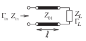
Figure \(\PageIndex{2}\): Transmission line of characteristic impedance \(Z_{01}\) terminated in a load with a reflection coefficient \(\Gamma_{L}\).

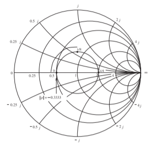
Figure \(\PageIndex{3}\): A Smith chart normalized to \(50\:\Omega\) with the input reflection coefficient locus of a \(50\:\Omega\) transmission line with a load of \(25\:\Omega\).

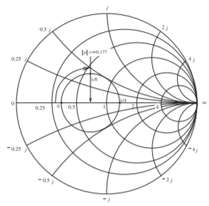
Figure \(\PageIndex{4}\): A Smith chart normalized to \(75\:\Omega\) with the input reflection coefficient locus of a \(50\:\Omega\) transmission line with a load of \(25\:\Omega\).

Example \(\PageIndex{1}\): Reflection Coefficient, Reference Impedance Change

In the circuit to the right, a \(50-\Omega\) lossless line is terminated in a \(25-\Omega\) load. Plot the locus, with respect to the length of the line, of the reflection coefficient looking into the line, referencing it first to a \(50-\Omega\) reference impedance and then to a \(75-\Omega\) reference impedance.

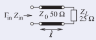
Figure \(\PageIndex{5}\)

Solution

Let the input reflection coefficient referenced to a \(50-\Omega\) system be \(\Gamma_{\text{in, }50}\), and when it is referenced to \(75-\Omega\) it is \(\Gamma_{\text{in, }75}\). In the \(50-\Omega\) system the reflection coefficient of the load is

\[\label{eq:7}\Gamma_{L, 50}=\frac{Z_{L}-50}{Z_{L}+50}=\frac{25-50}{25+50}=-0.3333 \]

and

\[\label{eq:8}\Gamma_{\text{in, }50}=\Gamma_{L, 50}\text{e}^{-\jmath 2\theta} \]

where \(\theta = (\beta\ell)\) is the electrical length of the line. The locus, with respect to electrical length, of \(\Gamma_{\text{in, }50}\) is plotted in Figure \(\PageIndex{3}\) as the length \(\ell\) ranges from \(0\) to \(\lambda /8\) to \(\lambda /2\), and completes the circle at \(\lambda /2\). Now

\[\label{eq:9}Z_{\text{in}}=50\frac{1+\Gamma_{\text{in, }50}}{1-\Gamma_{\text{in, }50}} \]

so that the \(75-\Omega\) reflection coefficient is

\[\label{eq:10}\Gamma_{\text{in, }75}=\frac{Z_{\text{in}}, 75}{Z_{\text{in}}+75} \]

The locus of this reflection coefficient is plotted on a polar plot in Figure \(\PageIndex{4}\). This locus is the plot of \(\Gamma_{\text{in, }75}\) as the electrical length of the line, \(\theta\), is varied from \(0\) to \(π\). The center of the circle in Figure \(\PageIndex{4}\) is taken from the chart and determined to be \(−0.177\).

A circle is defined by its center and its radius, and Equations ((1.239)) and ((1.240)) of [11], enable the circles for the locus of \(\Gamma_{\text{in, }Z01}\) and \(\Gamma_{\text{in, }Z02}\) to be related. \(\Gamma_{\text{in, }Z01}\) has a center \(C_{Z01}\) and a radius \(R_{Z01}\):

\[\label{eq:11}C_{Z01}=0\quad\text{and}\quad R_{Z01}=|\Gamma_{L, Z01}| \]

In Equation ((1.239)) of [11] \(C_{Z01}\) replaces the center \(C_{z}\) and \(|\Gamma_{L,Z01}|\) takes the place of the radius \(R_{z}\). Similarly the center of the \(\Gamma_{Z02}\) circle, \(C_{Z02}\), replaces \(C_{w}\) and the radius of the \(\Gamma_{Z02}\) circle, \(R_{Z02}\), replaces \(R_{w}\). So the locus of the reflection coefficient referenced to \(Z_{02}\) is described by a circle with center and radius

\[\label{eq:12}C_{Z02}=\frac{B-A/C}{1-|C\text{T}_{L, Z01}|^{2}}+\frac{A}{C} \]

\[\label{eq:13}R_{Z02}=\left|\frac{(BC-A)\Gamma_{L, Z01}}{1-|C\text{T}_{L, Z01}|^{2}}\right| \]

Since, from Equation \(\eqref{eq:6}\), \(A = 1\) and \(B = C\) (\(B\) is given in Equation \(\eqref{eq:6}\)), this further simplifies to

\[\label{eq:14}C_{Z02}=\frac{B-1/B}{1-|B\Gamma_{L, Z01}|^{2}}+\frac{1}{B} \]

\[\label{eq:15}R_{Z02}=\left|\frac{(B^{2}-1)\Gamma_{L, Z01}}{1-|B\Gamma_{L, Z01}|^{2}}\right| \]

So the locus (with respect to frequency) of the input reflection coefficient of a terminated transmission line (of characteristic impedance \(Z_{01}\)) is a circle no matter what normalization impedance is used and the center of the circle will be on the real axis, the horizontal axis of the Smith chart.

Example \(\PageIndex{2}\): Center of Reflection Coefficient Locus

In Example \(\PageIndex{1}\) the locus of the input reflection coefficient referenced to \(75\:\Omega\) was plotted for a \(50-\Omega\) line terminated in a load with reflection coefficient (in the \(50-\Omega\) system) of \(−1/3\). Calculate the center of the input reflection coefficient when it is referenced to \(75\:\Omega\).

Solution

The center of the reflection coefficient normalized to \(Z_{01}\) is zero, that is, \(C_{50} = 0\). From Equation \(\eqref{eq:14}\), the center of the reflection coefficient normalized to \(Z_{02} = 75\:\Omega\) is

\[\label{eq:16}C_{75}=\frac{B-1/B}{1-|B\Gamma_{L, 50}|^{2}}+\frac{1}{B} \]

where

\[\label{eq:17}B=\frac{Z_{01}-Z_{02}}{Z_{01}+Z_{02}}=\frac{50-75}{50+75}=-0.2 \]

So

\[\label{eq:18}C_{75}=\frac{-0.2+5}{1-(0.2/3)^{2}}-5=-0.17857 \]

which compares favorably to a center of \(−0.177\) determined manually from the polar plot in the previous example.

3.5.3 Reflection Coefficient Locus

The direction of the locus of the input reflection coefficient of a terminated transmission line is always clockwise with increasing frequency, even if the Smith chart uses a reference or normalization impedance different from the characteristic impedance of the line. In Figure \(\PageIndex{6}\), \(Z_{01}\) is the characteristic impedance of the line and \(Z_{02}\) is the normalization impedance. The center of the circle of the reflection coefficient normalized to \(Z_{02}\) is to the left of the origin if \(Z_{02} > Z_{01}\), and to the right of the origin if normalized to \(Z_{02} < Z_{01}\), but always on the real axis.

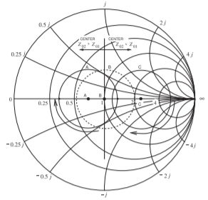
Figure \(\PageIndex{6}\): The locus of the input reflection coefficient normalized to \(Z_{02}\) of a terminated line of characteristic impedance \(Z_{01}\). The locus is with respect to the electrical length of the line and the arrows show the direction of rotation of the reflection coefficient. (Note that for the same terminating impedance the radii will also change, but this is not shown here.)

3.5.4 Summary

Smith charts are indispensable tools for RF and microwave engineers. Even with the ready availability of CAD programs. Smith charts are generally preferred for portraying measured and calculated data because of the easy interpretation of \(S\) parameters. With experience, the properties of circuits can be inferred. Also, with experience they are an invaluable design tool enabling the designer to see the beginning and endpoints of a design and infer the type of circuitry required to go from start to finish.

Footnotes

[1] These are not the cascadable \(ABCD\) parameters, but simply the coefficients commonly used with bilinear transforms.