5.8: Magnetic Transformer

In this section the use of magnetic transformers in microwave circuits will be discussed. Magnetic transformers can be used directly up to a few hundred megahertz or so, but the same transforming properties can be achieved using coupled transmission lines.

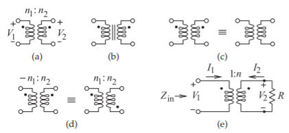
Figure \(\PageIndex{1}\): Magnetic transformers: (a) a transformer as two magnetically coupled windings with \(n_{1}\) windings on the primary (on the left) and \(n_{2}\) windings on the secondary (on the right) (the dots indicate magnetic polarity so that the voltages \(V_{1}\) and \(V_{2}\) have the same sign); (b) a magnetic transformer with a magnetic core; (c) identical representations of a magnetic transformer with the magnetic polarity implied for the transformer on the right; (d) two equivalent representations of a transformer having opposite magnetic polarities (an inverting transformer); and (e) a magnetic transformer circuit.

5.8.1 Properties of a Magnetic Transformer

A magnetic transformer (see Figure \(\PageIndex{1}\)) magnetically couples the current in one wire to current in another. The effect is amplified using coils of wires and using a core of magnetic material (material with high permeability) to create greater magnetic flux density. When coils are used, the symbol shown in Figure \(\PageIndex{1}\)(a) is used, with one of the windings called the primary winding and the other called the secondary winding. If there is a magnetic core around which the coils are wound, then the symbol shown in Figure \(\PageIndex{1}\)(b) is used, with the vertical lines indicating the core. However, even if there is a core, the simpler transformer symbol in Figure \(\PageIndex{1}\)(a) is more commonly used. Magnetic cores are useful up to several hundred megahertz and rely on the alignment of magnetic dipoles in the core material. Above a few hundred megahertz the magnetic dipoles cannot react quickly enough and so the core looks like an open circuit to magnetic flux. Thus the core is not useful for magnetically coupling signals above a few hundred megahertz. As mentioned, the dots above the coils in Figure \(\PageIndex{1}\)(a) indicate the polarity of the magnetic flux with respect to the currents in the coils so that, as shown, \(V_{1}\) and \(V_{2}\) will have the same sign. Even if the magnetic polarity is not specifically shown, it is implied (see Figure \(\PageIndex{1}\)(c)). There are two ways of showing inversion of the magnetic polarity, as shown in Figure \(\PageIndex{1}\)(d), where a negative number of windings indicates opposite magnetic polarity.

The interest in using magnetic transformers in high-frequency circuit design is that configurations of magnetic transformers can be realized using coupled transmission lines to extend operation to hundreds of gigahertz. The transformer is easy to conceptualize, so it is convenient to first develop a circuit using the transformer and then translate it to transmission line form.

That is, in “back-of-the-envelope” microwave design, transformers can be used to indicate coupling, with the details of the coupling left until later when the electrical design is translated into a physical design. Restrictions must be followed as not all transformer configurations can be translated this way. Transformer characteristics are developed below.

The following notation is used with a magnetic transformer:

\(L_{1},\: L_{2}\): the self-inductances of the two coils

\(M\): the mutual inductance

\(k\): the coupling factor,

\[\label{eq:1}k=\frac{M}{\sqrt{L_{1}L_{2}}} \]

Referring to Figure \(\PageIndex{1}\)(e), the voltage transformer ratio is

\[\label{eq:2}V_{2}=nV_{1} \]

where \(n\) is the ratio of the number of secondary to primary windings. An ideal transformer has “perfect coupling,” indicated by \(k = 1\), and the self-inductances are proportional to the square of the number of windings, so

\[\label{eq:3}\frac{V_{2}}{V_{1}}=\sqrt{\frac{L_{2}}{L_{1}}} \]

The general equation relating the currents of the circuit in Figure \(\PageIndex{1}\)(e) is

\[\label{eq:4} RI_{2} +\jmath\omega L_{2}I_{2} + \jmath\omega MI_{1} = 0 \]

and so

\[\label{eq:5}\frac{I_{1}}{I_{2}}=-\frac{R+\jmath\omega L_{2}}{\jmath\omega M} \]

If \(R ≪ \omega L_{2}\), then the current transformer ratio is

\[\label{eq:6}\frac{I_{1}}{I_{2}}\approx -\frac{L_{2}}{M}=-\sqrt{\frac{L_{2}}{L_{1}}} \]

Notice that combining Equations \(\eqref{eq:3}\) and \(\eqref{eq:6}\) leads to calculation of the transforming effect on impedance. On the Coil \(\mathsf{1}\) side, the input impedance is (referring to Figure 5-19(e))

\[\label{eq:7}Z_{\text{in}}=\frac{V_{1}}{I_{1}}=-\frac{V_{2}}{I_{2}}\left(\frac{L_{1}}{L_{2}}\right)=R\frac{L_{1}}{L_{2}} \]

In practice, however, there is always some magnetic field leakage—not all of the magnetic field created by the current in Coil \(\mathsf{1}\) goes through (or links) Coil \(\mathsf{2}\)—and so \(k < 1\). Then from Equations \(\eqref{eq:3}\)–\(\eqref{eq:7}\),

\[\begin{align}\label{eq:8}V_{1}&=\jmath\omega L_{1}I_{1}+\jmath\omega I_{2}\\ \label{eq:9}0&=RI_{2}+\jmath\omega L_{2}I_{2}+\jmath\omega MI_{1}\end{align} \]

Again, assuming that \(R ≪ \omega L_{2}\), a modified expression for the input impedance is obtained that accounts for nonideal coupling:

\[\label{eq:10}Z_{\text{in}}=R\frac{L_{1}}{L_{2}}+\jmath\omega L_{1}(1-k^{2}) \]

Imperfect coupling, \(k < 1\), causes the input impedance to be reactive and this limits the bandwidth of the transformer. Stray capacitance is another factor that impacts the bandwidth of the transformer.

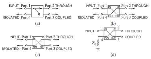
Figure \(\PageIndex{2}\): Commonly used symbols for hybrids: (a) through and coupled ports; (b) \(180^{\circ}\) hybrid; (c) \(90^{\circ}\) hybrid; and (d) hybrid with the isolated port terminated in a matched load.