7.2: Fano-Bode Limits
- Page ID
- 41144
\( \newcommand{\vecs}[1]{\overset { \scriptstyle \rightharpoonup} {\mathbf{#1}} } \)
\( \newcommand{\vecd}[1]{\overset{-\!-\!\rightharpoonup}{\vphantom{a}\smash {#1}}} \)
\( \newcommand{\id}{\mathrm{id}}\) \( \newcommand{\Span}{\mathrm{span}}\)
( \newcommand{\kernel}{\mathrm{null}\,}\) \( \newcommand{\range}{\mathrm{range}\,}\)
\( \newcommand{\RealPart}{\mathrm{Re}}\) \( \newcommand{\ImaginaryPart}{\mathrm{Im}}\)
\( \newcommand{\Argument}{\mathrm{Arg}}\) \( \newcommand{\norm}[1]{\| #1 \|}\)
\( \newcommand{\inner}[2]{\langle #1, #2 \rangle}\)
\( \newcommand{\Span}{\mathrm{span}}\)
\( \newcommand{\id}{\mathrm{id}}\)
\( \newcommand{\Span}{\mathrm{span}}\)
\( \newcommand{\kernel}{\mathrm{null}\,}\)
\( \newcommand{\range}{\mathrm{range}\,}\)
\( \newcommand{\RealPart}{\mathrm{Re}}\)
\( \newcommand{\ImaginaryPart}{\mathrm{Im}}\)
\( \newcommand{\Argument}{\mathrm{Arg}}\)
\( \newcommand{\norm}[1]{\| #1 \|}\)
\( \newcommand{\inner}[2]{\langle #1, #2 \rangle}\)
\( \newcommand{\Span}{\mathrm{span}}\) \( \newcommand{\AA}{\unicode[.8,0]{x212B}}\)
\( \newcommand{\vectorA}[1]{\vec{#1}} % arrow\)
\( \newcommand{\vectorAt}[1]{\vec{\text{#1}}} % arrow\)
\( \newcommand{\vectorB}[1]{\overset { \scriptstyle \rightharpoonup} {\mathbf{#1}} } \)
\( \newcommand{\vectorC}[1]{\textbf{#1}} \)
\( \newcommand{\vectorD}[1]{\overrightarrow{#1}} \)
\( \newcommand{\vectorDt}[1]{\overrightarrow{\text{#1}}} \)
\( \newcommand{\vectE}[1]{\overset{-\!-\!\rightharpoonup}{\vphantom{a}\smash{\mathbf {#1}}}} \)
\( \newcommand{\vecs}[1]{\overset { \scriptstyle \rightharpoonup} {\mathbf{#1}} } \)
\( \newcommand{\vecd}[1]{\overset{-\!-\!\rightharpoonup}{\vphantom{a}\smash {#1}}} \)
\(\newcommand{\avec}{\mathbf a}\) \(\newcommand{\bvec}{\mathbf b}\) \(\newcommand{\cvec}{\mathbf c}\) \(\newcommand{\dvec}{\mathbf d}\) \(\newcommand{\dtil}{\widetilde{\mathbf d}}\) \(\newcommand{\evec}{\mathbf e}\) \(\newcommand{\fvec}{\mathbf f}\) \(\newcommand{\nvec}{\mathbf n}\) \(\newcommand{\pvec}{\mathbf p}\) \(\newcommand{\qvec}{\mathbf q}\) \(\newcommand{\svec}{\mathbf s}\) \(\newcommand{\tvec}{\mathbf t}\) \(\newcommand{\uvec}{\mathbf u}\) \(\newcommand{\vvec}{\mathbf v}\) \(\newcommand{\wvec}{\mathbf w}\) \(\newcommand{\xvec}{\mathbf x}\) \(\newcommand{\yvec}{\mathbf y}\) \(\newcommand{\zvec}{\mathbf z}\) \(\newcommand{\rvec}{\mathbf r}\) \(\newcommand{\mvec}{\mathbf m}\) \(\newcommand{\zerovec}{\mathbf 0}\) \(\newcommand{\onevec}{\mathbf 1}\) \(\newcommand{\real}{\mathbb R}\) \(\newcommand{\twovec}[2]{\left[\begin{array}{r}#1 \\ #2 \end{array}\right]}\) \(\newcommand{\ctwovec}[2]{\left[\begin{array}{c}#1 \\ #2 \end{array}\right]}\) \(\newcommand{\threevec}[3]{\left[\begin{array}{r}#1 \\ #2 \\ #3 \end{array}\right]}\) \(\newcommand{\cthreevec}[3]{\left[\begin{array}{c}#1 \\ #2 \\ #3 \end{array}\right]}\) \(\newcommand{\fourvec}[4]{\left[\begin{array}{r}#1 \\ #2 \\ #3 \\ #4 \end{array}\right]}\) \(\newcommand{\cfourvec}[4]{\left[\begin{array}{c}#1 \\ #2 \\ #3 \\ #4 \end{array}\right]}\) \(\newcommand{\fivevec}[5]{\left[\begin{array}{r}#1 \\ #2 \\ #3 \\ #4 \\ #5 \\ \end{array}\right]}\) \(\newcommand{\cfivevec}[5]{\left[\begin{array}{c}#1 \\ #2 \\ #3 \\ #4 \\ #5 \\ \end{array}\right]}\) \(\newcommand{\mattwo}[4]{\left[\begin{array}{rr}#1 \amp #2 \\ #3 \amp #4 \\ \end{array}\right]}\) \(\newcommand{\laspan}[1]{\text{Span}\{#1\}}\) \(\newcommand{\bcal}{\cal B}\) \(\newcommand{\ccal}{\cal C}\) \(\newcommand{\scal}{\cal S}\) \(\newcommand{\wcal}{\cal W}\) \(\newcommand{\ecal}{\cal E}\) \(\newcommand{\coords}[2]{\left\{#1\right\}_{#2}}\) \(\newcommand{\gray}[1]{\color{gray}{#1}}\) \(\newcommand{\lgray}[1]{\color{lightgray}{#1}}\) \(\newcommand{\rank}{\operatorname{rank}}\) \(\newcommand{\row}{\text{Row}}\) \(\newcommand{\col}{\text{Col}}\) \(\renewcommand{\row}{\text{Row}}\) \(\newcommand{\nul}{\text{Nul}}\) \(\newcommand{\var}{\text{Var}}\) \(\newcommand{\corr}{\text{corr}}\) \(\newcommand{\len}[1]{\left|#1\right|}\) \(\newcommand{\bbar}{\overline{\bvec}}\) \(\newcommand{\bhat}{\widehat{\bvec}}\) \(\newcommand{\bperp}{\bvec^\perp}\) \(\newcommand{\xhat}{\widehat{\xvec}}\) \(\newcommand{\vhat}{\widehat{\vvec}}\) \(\newcommand{\uhat}{\widehat{\uvec}}\) \(\newcommand{\what}{\widehat{\wvec}}\) \(\newcommand{\Sighat}{\widehat{\Sigma}}\) \(\newcommand{\lt}{<}\) \(\newcommand{\gt}{>}\) \(\newcommand{\amp}{&}\) \(\definecolor{fillinmathshade}{gray}{0.9}\)
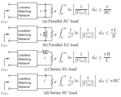
Figure \(\PageIndex{1}\): Fano-Bode limits for circuits with reactive loads.
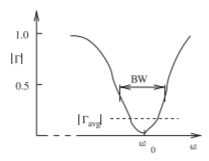
Figure \(\PageIndex{2}\): Response looking into matching network used in defining nonintegral Fano-Bode criteria. The bandwidth of the passband (low \(\Gamma\), is BW).
A complex load having energy storage elements limits the bandwidth of the match achieved by a matching network. Theoretical limits addressing the bandwidth and the quality of the match were developed by Fano [1, 2] based on earlier work by Bode [3]. These theoretical limits are known as the FanoBode criteria or the Fano-Bode limits. The limits for simple loads are shown in Figure \(\PageIndex{1}\). More general loads are treated by Fano [1]. The Fano-Bode criteria are used to justify the broad assertion that the more reactive energy stored in a load, the narrower the bandwidth of a match.
The Fano-Bode criteria include the term \(1/ |\Gamma (\omega )|\), which is the inverse of the magnitude of the reflection coefficient looking into the matching network, as shown in Figure \(\PageIndex{1}\). A matching network provides matching over a radian bandwidth BW, and outside the matching frequency band the magnitude of the reflection coefficient approaches \(1\). Introducing \(\Gamma_{\text{avg}}\) as the average absolute value of \(\Gamma (\omega )\) within the passband, and with \(f_{0} = \omega_{0}/(2\pi )\) as the center frequency of the match (see Figure \(\PageIndex{2}\)), then the four Fano-Bode criteria shown in Figure \(\PageIndex{1}\) can be written as
Parallel RC load:
\[\label{eq:1}\frac{\text{BW}}{\omega_{0}}\ln\left(\frac{1}{\Gamma_{\text{avg}}}\right)\leq\frac{\pi}{R(\omega_{0}C)} \]
Parallel RL load:
\[\label{eq:2}\frac{\text{BW}}{\omega_{0}}\ln\left(\frac{1}{\Gamma_{\text{avg}}}\right)\leq\frac{\pi(\omega_{0}L)}{R} \]
Series RL load:
\[\label{eq:3}\frac{\text{BW}}{\omega_{0}}\ln\left(\frac{1}{\Gamma_{\text{avg}}}\right)\leq\frac{\pi R}{(\omega_{0} L)} \]
Series RC load:
\[\label{eq:4}\frac{\text{BW}}{\omega_{0}}\ln\left(\frac{1}{\Gamma_{\text{avg}}}\right)\leq\pi R(\omega_{0}C) \]
In terms of reactance and susceptance these can be written as
Parallel load:
\[\label{eq:5}\frac{\text{BW}}{\omega_{0}}\ln\left(\frac{1}{\Gamma_{\text{avg}}}\right)\leq\frac{\pi G}{|B|} \]
Series load:
\[\label{eq:6}\frac{\text{BW}}{\omega_{0}}\ln\left(\frac{1}{\Gamma_{\text{avg}}}\right)\leq\frac{\pi R}{|X|} \]
where \(G = 1/R\) is the conductance of the load, \(B\) is the load susceptance, and \(X\) is the load reactance. \(\text{BW}/\omega_{0}\) is the fractional bandwidth of the matching network. Equations \(\eqref{eq:5}\) and \(\eqref{eq:6}\) indicate that the greater the proportion of energy stored reactively in the load compared to the power dissipated in the load, the smaller the fractional bandwidth \((\text{BW}/\omega_{0})\) for the same average in-band reflection coefficient \(\Gamma_{\text{avg}}\).
Equations \(\eqref{eq:5}\) and \(\eqref{eq:6}\) can be simplified one step further:
\[\label{eq:7}\frac{\text{BW}}{\omega_{0}}\ln\left(\frac{1}{\Gamma_{\text{avg}}}\right)\leq\frac{\pi}{Q} \]
where \(Q\) is that of the load. Several general results can be drawn from Equation \(\eqref{eq:7}\) as follows:
- If the load stores any reactive energy, so that the \(Q\) of the load is nonzero, the in-band reflection coefficient looking into the matching network cannot be zero across the passband.
- The higher the \(Q\) of the load, the narrower the bandwidth of the match for the same average in-band reflection coefficient.
- The higher the \(Q\) of the load, the more difficult it will be to design the matching network to achieve a specified matching bandwidth.
- A match over all frequencies is only possible if the \(Q\) of the load is zero; that is, if the load is resistive. In this case a resistive load could be matched to a resistive source by using a magnetic transformer. Using a matching network with lumped \(L\) and \(C\) components will result in a match over a finite bandwidth. However, with more than two \(L\) and \(C\) elements the bandwidth of the match can be increased.
- Multielement matching networks are required to maximize the matching network bandwidth and minimize the in-band reflection coefficient. The matching network design becomes more difficult as the \(Q\) of the load increases.