7.3: Constant \(Q\) Circles

Last updated
Save as PDF

Page ID: 41145

\( \newcommand{\vecs}[1]{\overset { \scriptstyle \rightharpoonup} {\mathbf{#1}} } \) \( \newcommand{\vecd}[1]{\overset{-\!-\!\rightharpoonup}{\vphantom{a}\smash {#1}}} \)\(\newcommand{\id}{\mathrm{id}}\) \( \newcommand{\Span}{\mathrm{span}}\) \( \newcommand{\kernel}{\mathrm{null}\,}\) \( \newcommand{\range}{\mathrm{range}\,}\) \( \newcommand{\RealPart}{\mathrm{Re}}\) \( \newcommand{\ImaginaryPart}{\mathrm{Im}}\) \( \newcommand{\Argument}{\mathrm{Arg}}\) \( \newcommand{\norm}[1]{\| #1 \|}\) \( \newcommand{\inner}[2]{\langle #1, #2 \rangle}\) \( \newcommand{\Span}{\mathrm{span}}\) \(\newcommand{\id}{\mathrm{id}}\) \( \newcommand{\Span}{\mathrm{span}}\) \( \newcommand{\kernel}{\mathrm{null}\,}\) \( \newcommand{\range}{\mathrm{range}\,}\) \( \newcommand{\RealPart}{\mathrm{Re}}\) \( \newcommand{\ImaginaryPart}{\mathrm{Im}}\) \( \newcommand{\Argument}{\mathrm{Arg}}\) \( \newcommand{\norm}[1]{\| #1 \|}\) \( \newcommand{\inner}[2]{\langle #1, #2 \rangle}\) \( \newcommand{\Span}{\mathrm{span}}\)\(\newcommand{\AA}{\unicode[.8,0]{x212B}}\)

One strategy for wideband matching is based on the concept of matching to an intermediate resistance that is the geometric mean of the source and load impedances. This concept was introduced in Section 6.6 and can be generalized to intermediate impedances and can be represented on a Smith chart using constant \(Q\) as shown in Figure \(\PageIndex{1}\). If the load and source impedances, \(R_{L}\) and \(R_{S}\), are resistive, then the normalizing resistance \((R_{v})\) of the Smith chart should (although it is not necessary) be chosen as the geometric mean of the source and load resistance (i.e., \(R_{v} =\sqrt{R_{L}R_{S}}\)). To maintain a specific circuit \(Q\), and hence bandwidth, the locus of impedances in the design must stay within or touch, the corresponding constant \(Q\) circle.

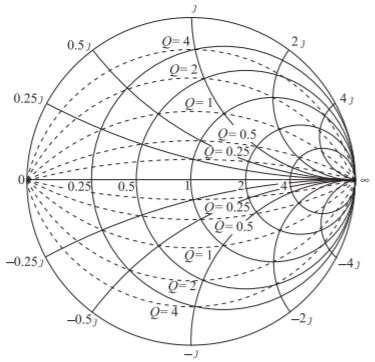
Figure \(\PageIndex{1}\): Impedance Smith chart with constant \(Q\) circles.

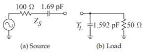
Figure \(\PageIndex{2}\): Matching problem in Example \(\PageIndex{1}\).

Example \(\PageIndex{1}\): Broadband Matching Using Constant \(Q\) Circles

Design a broadband matching network at \(1\text{ GHz}\) for the situation shown in Figure \(\PageIndex{2}\).

Solution

\(Z_{S} = 100 −\jmath 94.25\:\Omega,\: Y_{L} = 0.02 +\jmath 0.01\text{ S}\), and \(Z_{L} = 40.0 −\jmath 20.0\:\Omega\). Normalizing these to \(100\:\Omega\) results in \(z_{S} = 1 −\jmath 0.9425,\: y_{L} = 2+ \jmath 1,\) and \(z_{L} = 0.400 −\jmath 0.200\). Also the \(Q\) of the source, \(Q_{S} = 0.9425\) and the \(Q\) of the load is \(Q_{L} = 0.500\). The matching design puts a network in front of \(z_{L}\) to present an impedance \(z_{S}^{\ast}\) to the source. These values are plotted in Figure \(\PageIndex{3}\). The design objective is to maintain maximum bandwidth and this is done by staying inside the \(Q = 0.9425\) circle, where the \(Q\) is the larger of the source and load \(Q\)s.

Design can proceed by moving back from the load toward the source, or from the source to the load. Most commonly the perspective used is moving back from the load. Then the load \(z_{L}\) is transformed to \(z_{S}^{\ast}\). Maximum bandwidth is approximately achieved if the matching stages do not exceed the maximum \(Q\) of the load or of the source. So the \(Q\) of the stages cannot exceed \(0.9425\). An appropriate matching concept is shown in Figure \(\PageIndex{4}\). The locus is \(\mathsf{B}\to\mathsf{C}\to\mathsf{D}\to\mathsf{E}\to\mathsf{F}\to\mathsf{G}\to\mathsf{A}\). The matching network is therefore of the form shown in Figure \(\PageIndex{5}\). The rest of the design is extraction of numerical values, but the difficult part of the design has been done.

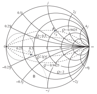
Figure \(\PageIndex{3}\): Impedance Smith chart indicating the matching problem in Example \(\PageIndex{1}\) with load and source plotted and their constant \(Q\) circles. The normalization impedance is \(100\:\Omega\).

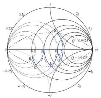
Figure \(\PageIndex{4}\): Outlining of matching concept in Example \(\PageIndex{1}\).

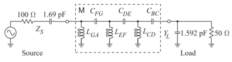
Figure \(\PageIndex{5}\): Matching network \(\mathsf{M}\) in Example \(\PageIndex{1}\).