
7.6: Matching a Series RC load
- Page ID
- 41148
The matching network design described in this section is appropriate for a real source impedance and series RC load where the load resistance is less than the source resistance. Also a two-section quarter-wave impedance transformer will be considered as this has performance that is representative of what is reasonable to achieve using transmission-line based impedance transformers. Tapers are not considered here as their particular advantage of an indefinite passband when matching resistive source and load impedance disappears when the load (or source) is reactive.
Design Examples
Figure \(\PageIndex{1}\)(a) presents the problem of matching to the input of a transistor which is modeled here as a capacitor in series with a resistive load. This is the typical model for the input of a FET.
With a two-section cascaded quarter-wave transformer an appropriate matching network is shown in Figure \(\PageIndex{2}\)(b). This topology is based on the design concepts shown in Figures \(\PageIndex{2}\)(c, d and e) where the single-frequency reflection coefficient loci with respect to increasing line length are shown. The overall concept is that line \(3\) rotates the load impedance to a resistance \(R_{X}\) and then \(R_{X}\) is matched to \(R_{S}\) using a two-section quarter-wave transformer,
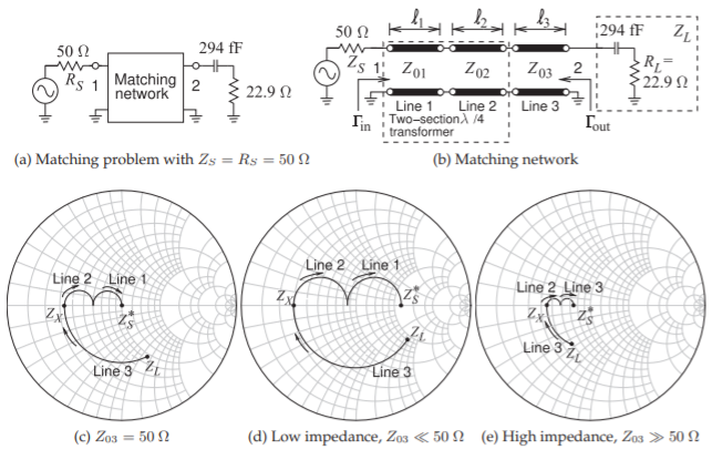
Figure \(\PageIndex{1}\): Matching problem of the case study of Section 7.6 using a two-section cascaded quarter-wave impedance transformer. The arrows in (c), (d), and (e) indicate increasing line length at \(10\text{ GHz}\). The Smith charts are normalized to \(Z_{03}\) and present three design concepts. (The choice of high \(Z_{03}\) is appropriate for \(R_{L} < Z_{S}\) and a capacitor in the load.)
that is, lines \(1\) and \(2\).
At \(10\text{ GHz}\) the \(294\text{ fF}\) capacitor has a reactance of \(−54.13\:\Omega\) and with the resistive part of the load the input of the transistor has a \(Q\) of \(2.36\). This is plotted on the \(50\:\Omega\) Smith chart in Figure \(\PageIndex{1}\)(c). The design concept is that line \(3\) rotates the load \(Z_{L}\) to a purely resistive load of \(10.0\:\Omega\). Then a \(\lambda/4\)-long line, line \(2\), rotates the reflection coefficient to an intermediate impedance, and this is followed by line \(1\), another \(\lambda/4\)-long line which takes the input impedance to \(50\:\Omega\). Note that the electrical lengths of the lines are given by the angle subtended by the arcs and do not correspond to the drawn lengths of the arcs. Here the electrical length of line \(1\) is \(50.0^{\circ}\) and that of lines \(2\) and \(3\) are \(90^{\circ}\).
Two alternative design concepts are shown in Figures \(\PageIndex{1}\)(d and e). Figure \(\PageIndex{1}\)(d) describes a low impedance \((Z_{03} ≪ 50\:\Omega)\) design concept. If \(Z_{03} = 20\:\Omega\) then the electrical length of the line is \(72.3^{\circ}\) and the intermediate impedance \(Z_{X} = 2.41\:\Omega\). An alternative is to use a high characteristic impedance for line \(3\) as outlined in Figure \(\PageIndex{1}\)(e). With \(Z_{03} = 100\:\Omega\) the electrical length of line \(3\) is \(29.4^{\circ}\) and \(Z_{X} = 17.54\:\Omega\). Of these three design concepts the third design concept with the highest \(Z_{03}\) is preferable on two accounts. One of these is that the electrical length of line \(3\) is the smallest, and since the electrical lengths of lines \(1\) and \(2\) are fixed (each is \(\lambda /8\) long), this results in the lowest overall electrical line length. Secondly the intermediate resistance is closest
| \(Z_{03}\) \((\Omega)\) |
\(\beta\ell_{3}\) | \(Z_{X}\) \((\Omega)\) |
\(Z_{02}\) \((\Omega)\) |
\(Z_{01}\) \((\Omega)\) |
\(0.1\text{ dB}\) Bandwidth \((\text{GHz}\) |
|
|---|---|---|---|---|---|---|
| \(10\) | \(81.1^{\circ}\) | \(0.65\) | \(1.92\) | \(18.86\) | \(9.90–10.18\: (0.28)\) | |
| \(20\) | \(72.3^{\circ}\) | \(2.41\) | \(5.14\) | \(23.4\) | \(9.76–10.25\: (0.49)\) | |
| \(30\) | \(64.1^{\circ}\) | \(4.86\) | \(8.70\) | \(27.9\) | \(9.69–10.39\: (0.70)\) | |
| \(40\) | \(56.6^{\circ}\) | \(7.50\) | \(9.62\) | \(31.1\) | \(9.62–10.46\: (0.84)\) | |
| \(50\) | \(50.0^{\circ}\) | \(10.0\) | \(9.55\) | \(33.4\) | \(9.55-10.52\: (0.97)\) | |
| \(60\) | \(44.4^{\circ}\) | \(12.2\) | \(17.3\) | \(35.1\) | \(9.54-10.53\: (0.99)\) | |
| \(70\) | \(39.6^{\circ}\) | \(14.0\) | \(19.2\) | \(36.3\) | \(9.48–10.60\: (1.11)\) | |
| \(80\) | \(35.6^{\circ}\) | \(15.4\) | \(20.7\) | \(37.3\) | \(9.48–10.60\: (1.11)\) | |
| \(90\) | \(32.3^{\circ}\) | \(16.6\) | \(21.9\) | \(38.0\) | \(9.48–10.60\: (1.11)\) | |
| \(100\) | \(29.4^{\circ}\) | \(17.5\) | \(22.8\) | \(38.5\) | \(9.48–10.60\: (1.11)\) | |
Table \(\PageIndex{1}\): Matching network performance with different \(Z_{03}\) with electrical length \(\beta\ell_{3}\). The minimum and maxium frequencies of the passband are when \(T = 0.989\), i.e. when the transmission loss is \(0.1\text{ dB}\).
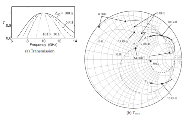
Figure \(\PageIndex{2}\): Characteristics of the matching network in Figure \(\PageIndex{1}\)(b) for \(Z_{03} = 10\:\Omega,\: 30\:\Omega,\: 50\:\Omega,\) and \(100\:\Omega\). The Smith chart in (b) is normalized to \(22.9\:\Omega\) and show the frequency loci of \(\Gamma_{\text{out}}\) for four matching network designs for \(Z_{03} = 10\:\Omega,\: 30\:\Omega,\: 50\:\Omega,\) and \(100\:\Omega\). The Smith chart also shows the frequency locus of \(Z_{L}\) and \(Z_{L}^{\ast}\). Note that \(\Gamma_{\text{out}}\) is equal to the reflection coefficient of \(Z_{L}^{\ast}\) at \(10\text{ GHz}\) for all matching networks.
to the complex conjugate of the source impedance, \(Z_{S}^{\ast}\), which of course is just \(Z_{S}\) here since the source is real.
Table \(\PageIndex{1}\) compares several trial designs with varying \(Z_{03}\) and it is apparent that the characteristic impedance of \(Z_{03}\) needs to be high. A maximum \(Z_{03}\) of \(100\:\Omega\) is typical of many transmission line technologies and especially of planar transmission lines like microstrip. Note that the maximum bandwidth is \(11\%\) which is considerably less than the approximately \(90\%\) bandwidth that could be obtained for a two-section quarter-wave transformer if the capacitance in the load was not present (see Table 7.5.3).
The transmission characteristics of the matching network designed using four values of \(Z_{03}\) ranging from \(10\:\Omega\) to \(100\:\Omega\) are shown in Figure \(\PageIndex{2}\)(a). Examination of the Smith chart plot, Figure \(\PageIndex{2}\)(b), reveals the fundamental problem in broadband matching of reactive loads to a resistive source impedance. First consider the frequency locus of the load \(Z_{L}\) which is seen to have a clockwise rotation on the Smith chart as is typical of nonresonant impedances. Matching requires that the impedance presented by the network at port \(2\) be the complex conjugate of \(Z_{L}\), i.e. \(Z_{L}^{\ast}\). \(Z_{L}^{\ast}\) is seen to rotate in the counter-clockwise direction with increasing frequency. The frequency loci of the reflection coefficients, \(\Gamma_{\text{out}}\), that are presented looking into port \(2\) of the matching network (in Figure \(\PageIndex{1}\)(a)) for each of the four designs are also plotted in Figure \(\PageIndex{2}\)(b). These all rotate in the clockwise direction so that it is only possible for these matching networks to present the desired impedance \(Z_{L}^{\ast}\) at a single frequency, here \(10\text{ GHz}\). The angular length of the \(\Gamma_{\text{out}}\) loci from \(6\text{ GHz}\) to \(14\text{ GHz}\) for the four designs differ.
The line with \(Z_{03} = 100\:\Omega\) has the shortest \(\Gamma_{\text{out}}\) locus having the shortest total angular length (and hence shortest electrical and physical lengths). The passband responses of the various designs are shown in Figure \(\PageIndex{2}\)(a) and the broadest passband response is obtained when \(Z_{03} = 100\:\Omega\) and this impedance is about the largest that could be tolerated for a planar line as otherwise the microstrip characteristic impedance is become close to the \(377\:\Omega\) free space and radiation (and this loss) from the microstrip line is starting to be significant.
7.6.1 Summary
The lessons learned from the design in this section can be generalized with the results shown in Table \(\PageIndex{2}\). While these results were obtained for a particular form of the load (a series RC load) they are a broad indication of
| \(0.1\text{ dB}\) max. transmission loss, \(\%\) bandwidth | |||||||||
|---|---|---|---|---|---|---|---|---|---|
| \(Z_{L}/Z_{S}\) | \(Q\) at \(f_{0}\) | ||||||||
| \(0\) | \(0.25\) | \(0.5\) | \(0.75\) | \(1.0\) | \(1.5\) | \(2.0\) | \(2.5\) | \(3.0\) | |
| \(0.10\) | \(50\) | \(37\) | \(31\) | \(27\) | \(23\) | \(18\) | \(14\) | \(12\) | \(10\) |
| \(0.25\) | \(59\) | \(47\) | \(38\) | \(31\) | \(26\) | \(19\) | \(14\) | \(11\) | \(9\) |
| \(0.50\) | \(85\) | \(56\) | \(45\) | \(34\) | \(27\) | \(19\) | \(14\) | \(11\) | \(8\) |
| \(0.75\) | \(\infty\) | \(78\) | \(50\) | \(36\) | \(27\) | \(18\) | \(13\) | \(9\) | \(7\) |
| \(1.00\) | \(\infty\) | \(116\) | \(56\) | \(37\) | \(27\) | \(17\) | \(11\) | \(8\) | \(6\) |
| \(0.2\text{ dB}\) max. transmission loss, \(\%\) bandwidth | |||||||||
| \(Z_{L}/Z_{S}\) | \(Q\) at \(f_{0}\) | ||||||||
| \(Z_{L}/Z_{S}\) | \(0\) | \(0.25\) | \(0.5\) | \(0.75\) | \(1.0\) | \(1.5\) | \(2.0\) | \(2.5\) | \(3.0\) |
| \(0.10\) | \(51\) | \(45\) | \(39\) | \(35\) | \(31\) | \(24\) | \(20\) | \(16\) | \(14\) |
| \(0.25\) | \(73\) | \(59\) | \(49\) | \(41\) | \(34\) | \(26\) | \(20\) | \(16\) | \(14\) |
| \(0.50\) | \(98\) | \(77\) | \(58\) | \(46\) | \(38\) | \(26\) | \(20\) | \(15\) | \(12\) |
| \(0.75\) | \(\infty\) | \(106\) | \(68\) | \(50\) | \(39\) | \(25\) | \(18\) | \(14\) | \(11\) |
| \(1.00\) | \(\infty\) | \(181\) | \(80\) | \(52\) | \(38\) | \(24\) | \(16\) | \(12\) | \(9\) |
| \(0.5\text{ dB}\) max. transmission loss, \(\%\) bandwidth | |||||||||
| \(Z_{L}/Z_{S}\) | \(Q\) at \(f_{0}\) | ||||||||
| \(Z_{L}/Z_{S}\) | \(0\) | \(0.25\) | \(0.5\) | \(0.75\) | \(1.0\) | \(1.5\) | \(2.0\) | \(2.5\) | \(3.0\) |
| \(0.10\) | \(66\) | \(58\) | \(52\) | \(46\) | \(42\) | \(34\) | \(29\) | \(24\) | \(21\) |
| \(0.25\) | \(96\) | \(77\) | \(65\) | \(56\) | \(49\) | \(38\) | \(31\) | \(25\) | \(21\) |
| \(0.50\) | \(187\) | \(108\) | \(82\) | \(66\) | \(55\) | \(40\) | \(30\) | \(24\) | \(19\) |
| \(0.75\) | \(\infty\) | \(>41\) | \(104\) | \(75\) | \(58\) | \(39\) | \(28\) | \(22\) | \(17\) |
| \(1.00\) | \(\infty\) | \(>33\) | \(150\) | \(83\) | \(60\) | \(37\) | \(26\) | \(19\) | \(14\) |
| \(1.0\text{ dB}\) max. transmission loss, \(\%\) bandwidth | |||||||||
| \(Z_{L}/Z_{S}\) | \(Q\) at \(f_{0}\) | ||||||||
| \(Z_{L}/Z_{S}\) | \(0\) | \(0.25\) | \(0.5\) | \(0.75\) | \(1.0\) | \(1.5\) | \(2.0\) | \(2.5\) | \(3.0\) |
| \(0.10\) | \(82\) | \(72\) | \(64\) | \(58\) | \(53\) | \(45\) | \(38\) | \(33\) | \(29\) |
| \(0.25\) | \(123\) | \(98\) | \(83\) | \(72\) | \(63\) | \(51\) | \(42\) | \(34\) | \(30\) |
| \(0.50\) | \(\infty\) | \(>38\) | \(114\) | \(88\) | \(74\) | \(55\) | \(42\) | \(34\) | \(27\) |
| \(0.75\) | \(\infty\) | \(>27\) | \(>47\) | \(172\) | \(82\) | \(55\) | \(40\) | \(31\) | \(24\) |
| \(1.00\) | \(\infty\) | \(>24\) | \(>43\) | \(160\) | \(88\) | \(53\) | \(37\) | \(27\) | \(21\) |
Table \(\PageIndex{2}\): Bandwidths achievable for various \(R_{L}/Z_{S}\) ratios and \(Q\)s using the two-section quarter-wave transformer of Figure \(\PageIndex{1}\)(b) and \(Z_{03} = 2Z_{S}\). The percentage bandwidth is calculated as \(100\) times the difference of the high and low frequencies of the passband divided by the ideal match frequency, \(f_{0}\). The notation \(>33\) indicates that the passband is at all frequencies above \(0.33f_{0}\) as for small impedance discontinuities and low \(Q\), the two-section transformer is close to being a linear taper. \(Q\) is inversely proportion to frequency. Transmission losses of \(0.1\text{ dB},\: 0.2\text{ dB},\: 0.5\text{ dB}\), and \(1.0\text{ dB}\) correspond to a maximum \(|\Gamma_{\text{in}}|\) in the passband of \(|\Gamma_{m}| = 0.151,\: 0.212,\: 0.330,\) and \(0.454\) respectively. (The same bandwidths are obtained with inverted values of \(R_{L}/Z_{S}\) but requires a different design concept for the matching network.)
what can be achieved without exploiting resonance in the matching network. (Resonance is a technique to obtain improved results and is be considered in Section 7.7.) The performance metrics in Table \(\PageIndex{2}\) are much more realistic than the Fano-Bode limits which could require lossless networks of infinite complexity, and only consider the average passband reflection coefficient rather than the maximum in-band reflection coefficient.
For example, with a factor of \(2\) difference between \(Z_{L}\) and \(Z_{S}\) and with a \(Q\) of \(1\), the fractional bandwidth that can be readily achieved is \(27\%,\: 55\%,\: 38\%,\) and \(74\%\) for maximum passband losses of \(0.1\text{ dB},\: 0.2\text{ dB},\: 0.5\text{ dB},\) and \(1\text{ dB}\) respectively. Since matching networks are not usually used for frequency selectivity (which is more appropriate for a filter), and since there will be multiple matching networks in a design, it is common to use a maximum transmission loss of \(0.1\text{ dB}\) as a passband criterion.
7.6.2 Matching using Cascaded Transmission Lines and Constant \(Q\) Circles
The stepped-impedance transformer designs utilizing quarter-wavelength-long lines can be very long. In this section the design of a stepped-impedance transmission line transformer with shortened lines is considered. Design is conceptually derived from the quarter-wave transformer but design choices are made based on constant \(Q\) circles.
First consider the single-line matching problem shown in Figure \(\PageIndex{3}\)(a). The normalized impedances are plotted on a Smith chart with constant \(Q\) circles in Figure \(\PageIndex{3}\)(b). A detailed view is given in Figure \(\PageIndex{3}\)(c) and this will be used to describe the design procedure. The normalizing reference impedance \(Z_{0}\) is arbitrary and does not need to be related to the source or load impedance, or to the characteristic impedance of the line.
Figure \(\PageIndex{4}\)(a) shows a quarter-wavelength-long transmission line matching a normalized load \(z_{L}\) to a normalized source impedance \(z_{S}\) with the arrow on the reflection coefficient locus indicating the direction of increasing line length. The arc subtends an angle of \(180^{\circ}\) corresponding to the line having an electrical length of \(90^{\circ}\), i.e. it is \(\lambda /4\) long. The maximum \(Q\) along the arc is near \(0.6\) indicating an approximate fractional bandwidth of \(1/Q\) or \(1.6\).
Greater bandwidth of the match can be obtained by using more line sections and matching to an intermediate impedance. This situation is shown in Figure \(\PageIndex{4}\)(b) where there are two quarter-wavelength-long transmission lines each matching to a normalized intermediate resistance \(r_{v} =\sqrt{z_{s}z_{L}}\) since both \(z_{s}\) and \(z_{L}\) are resistances. The two arcs in the locus each are part of a circle whose center can be used to determine the characteristic impedance of each of the lines. As an approximation, the center of the circle containing the arc for transmission line \(n\) is \(C_{n}\) referenced to the impedance \(Z_{0}\) and then \(Z_{0n}\approx Z_{0}(1 + 2C_{0n})\) (see Section 4.5). (Of course we already know that each of the lines is a quarter-wave transformer so \(Z_{01} = Z_{0}\sqrt{z_{s}r_{v}}\) and \(Z_{02} = Z_{0}\sqrt{z_{v}r_{L}}\)). The maximum \(Q\) set by the matching network is now \(0.28\) so the fractional bandwidth has increased to \(1/0.28 = 3.57\). This process can be continued indefinitely. With a matching network with three quarter-wave lines, as shown in Figure \(\PageIndex{4}\)(c) the maximum \(Q\) is further reduced and the fractional bandwidth increased.
The cascaded quarter-wave lines can reliably be used to obtain widebandwidth matching but the overall length of the network becomes quite
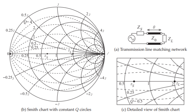
Figure \(\PageIndex{3}\): Transmission line matching a source impedance \(Z_{S}\) to a load impedance \(Z_{L}\).
large. A more compact matching network with shorter overall line length can be obtained using lines that are shorter than \(\lambda/4\). Such a network design is shown in Figure \(\PageIndex{4}\)(d) with electrical lengths of each of the three lines being less than that of a quarter-wave line (each is about \(\lambda/8\) long). The design problem then becomes one of determining the number of lines (or sections), determining the electrical lengths of the lines, the \(\Theta\)s, and then the characteristic impedance of the lines.
A reasonably good estimate can be obtained using a Smith chart and the constant \(Q\) circles. Generally maximum bandwidth is obtained if no one point on the locus sets the maximum circuit \(Q\). A better solution is when multiple arcs on the locus all touch the same \(Q\) line.
While the illustration used here has resistive load and source impedances the technique can be used with complex source and load impedances. The complicating factor is that if the source and/or load impedances have reactances, then the source and load impedances will vary with frequency. Still resistive matching provides a good initial point in a design and starting from here optimization in a microwave circuit simulator can be used to finalize a design. A good approach is to absorb the impedance variation with frequency into the matching network.
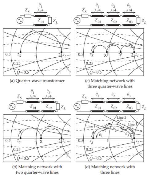
Figure \(\PageIndex{4}\): Broadband cascaded line matching networks. The arrows in the Smith chart locus indicate the direction with increasing line length.