1.6: Electric and Magnetic Field Laws

Before Maxwell’s equations were postulated, several laws of electromagnetics were known. These are the Biot–Savart law, Ampere’s circuital law, Gauss’s law, Gauss’s law for magnetism, and Faraday’s law. The laws are for specific circumstances and mostly for static fields. In this section they are

1.6.1 Ampere's Circuital Law

Ampere’s circuital law, often called just Ampere’s law, relates direct current and the static magnetic field \(\overline{H}\). The relationship is based on Figure \(\PageIndex{1}\). In the static situation, \(\partial \overline{D}/\partial t= 0\), and so one of Maxwell’s equations, Equation (1.5.36), reduces to

\[\label{eq:1}\oint_{\ell}\overline{H}\cdot d\ell =I_{\text{enclosed}} \]

This is Ampere’s circuital law.

1.6.2 Biot-Savart Law

The Biot–Savart law relates current to static magnetic field. With \(\partial\mathbf{D}/\partial t = 0\), Equation (1.5.3) becomes

\[\label{eq:2}\nabla\times\overline{H}=\overline{J} \]

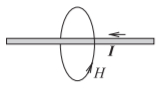
Figure \(\PageIndex{1}\): Diagram illustrating Ampere’s law. Ampere’s law relates the current on a wire to the magnetic field around it.

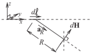
Figure \(\PageIndex{2}\): Diagram illustrating the Biot–Savart law. The Biot–Savart law relates current to magnetic field.

In Cartesian coordinates,

\[\label{eq:3}\nabla\times\overline{H}=\left(\frac{\partial H_{z}}{\partial y}-\frac{\partial H_{y}}{\partial z}\right)\hat{\mathbf{x}} +\left(\frac{\partial H_{x}}{\partial z}-\frac{\partial H_{z}}{\partial x}\right)\hat{\mathbf{y}}+\left(\frac{\partial H_{y}}{\partial x}-\frac{\partial H_{x}}{\partial y}\right)\hat{\mathbf{z}} \]

and if the current is confined to a thin wire as shown in Figure \(\PageIndex{2}\), \(\nabla\times\overline{H}\) reduces to an operation along the wire, but also with vector information. So the first step in the development of the Biot–Savart law, Equation \(\eqref{eq:2}\), is simplified to (ignoring vector information for now)

\[\label{eq:4}\frac{\partial H}{\partial\ell}=\frac{I}{4\pi R^{2}} \]

With vector information and moving the infinitesimal length of wire, \(d\ell\), from the left side of the equation to the right, the final form of the Biot–Savart law is obtained:

\[\label{eq:5}d\overline{H}=\frac{Id\ell\times\hat{\mathbf{a}}_{R}}{4\pi R^{2}} \]

which has the units of amps per meter in the SI system. In Equation \(\eqref{eq:5}\), \(I\) is current, \(d\ell\) is a length increment of a filament of current \(I\), \(\hat{\mathbf{a}}_{R}\) is the unit vector in the direction from the current filament to the magnetic field, and \(R\) is the distance between the filament and the magnetic field increment. So Equation \(\eqref{eq:5}\) is saying that a filament of current produces a magnetic field at a point. The total static magnetic field from a current on a wire or surface can be found by modeling the wire or surface as a number of current filaments, and the total magnetic field at a point is obtained by summing up the contributions from each filament.

1.6.3 Gauss's Law

The third law is Gauss’s law, which relates the static electric flux density vector, \(\mathbf{D}\), to charge. With reference to Figure \(\PageIndex{3}\), Gauss’s law in integral form is

\[\label{eq:6}\oint_{s}\overline{D}=\int_{v}\rho_{v} dv=Q_{\text{enclosed}} \]

which states that the integral of the electric flux density vector, \(\overline{D}\), is equal to the total charge enclosed by the surface, \(Q_{\text{enclosed}}\). This is just the integral form of the third Maxwell equation (Equation (1.5.37)).

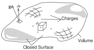
Figure \(\PageIndex{3}\): Diagram illustrating Gauss’s law. Charges are distributed in the volume enclosed by the closed surface. An incremental area is described by the vector \(d\mathbf{s}\) which is normal to the surface and whose magnitude is the area of the incremental area.

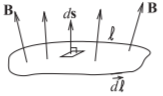
Figure \(\PageIndex{4}\): Diagram illustrating Faraday’s law. The contour \(\ell\) encloses the surface.

There is a similar law called Coulomb’s law which says that the magnitude of the force between two stationary point charges is directly proportional to the product of the magnitudes of charges and inversely proportional to the square of the distance between them. This law can be derived from Gauss’s law but is less general. Coulomb’s law applies only to stationary charges whereas with Gauss’s law the charges can be moving.

Gauss’s law has also been used for magnetic field where it is called Gauss’s law for magnetism. In integral form Gauss’s law for magnetism is

\[\label{eq:7}\oint_{s}\overline{B}=0 \]

where \(\overline{B}\), is the static magnetic flux density. This law is the same as saying that there are no magnetic charges. “Gauss’s law for magnetism” is a name that is not universally used and many people simply say that there are no magnetic charges.

1.6.4 Faraday's Law

Faraday’s law relates a time-varying magnetic field to an induced voltage drop, \(V\), which is now understood to be \(\oint_{\ell}E\cdot d\ell\), that is, the closed contour integral of the electric field,

\[\label{eq:8}V=\oint_{\ell}\overline{\mathcal{E}}\cdot d\ell =-\oint_{s}\frac{\partial\overline{\mathcal{B}}}{\partial t}\cdot d\mathbf{s} \]

and this has the units of volts in the SI unit system. This is just the first of Maxwell’s equations in integral form (see Equation (1.5.35)). The operation described in Equation \(\eqref{eq:8}\) is illustrated in Figure \(\PageIndex{4}\).