
1.8: Electric and Magnetic Walls
- Page ID
- 41009

The boundaries imposed by conductors and the interface between dielectrics define the mode structure (i.e., orientation of the fields) supported by a transmission line. Understanding the fields at the interfaces provides the intuition required to understand the operational frequency limits of distributed structures such as transmission lines.
1.8.1 Electric Wall
An electric wall is formed by an ideal conductor, as shown in Figure \(\PageIndex{1}\), where there are electric charges at the surface of the conductor. Consider that the conductor in Figure \(\PageIndex{1}\)(a) carries a current of density \(J\) and charge of density \(\rho_{V}\). As the conductivity of the conductor goes to infinity, the conductor becomes a perfect conductor and forms an electric wall, as shown in Figure \(\PageIndex{1}\)(b). The current and charge now occupy the very skin of the conductor at the interface to the region above which there is either free space or a dielectric. The behavior of the fields at the interface can be understood
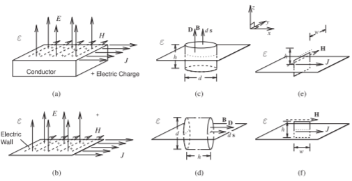
Figure \(\PageIndex{1}\): Properties of an electric wall: (a) the electrical field is perpendicular to a conductor and the magnetic field is parallel to it and is orthogonal to the current; (b) a conductor can be approximated by an electric wall; (c) cylinder used in deriving the normal electric field; (d) cylinder used in showing that the tangential electric field is zero; (e) contour used in deriving the tangential magnetic field in the \(y\) direction; and (f) contour used in deriving the \(z\)- and \(x\)-directed magnetic fields (they are zero).
by considering the integration surfaces and volumes shown in Figure \(\PageIndex{1}\)(c and d). The cylinder in Figure \(\PageIndex{1}\)(c) with height \(h\) and diameter \(d\) enables Gauss’s law (Equation (1.6.6)) to be applied. As \(h\longrightarrow 0\) (\(h\) approaching zero), Equation (1.6.6) yields
\[\label{eq:1}\oint_{s}\overline{\mathcal{D}}d\mathbf{s}=D_{z}\frac{1}{4}\pi d^{2}=\int_{v}\rho_{v}dv=Q_{\text{enclosed}}=\rho_{S}\frac{1}{4}\pi d^{2} \]
where \(\rho_{S}\) is the surface charge density (in SI units of \(\text{C/m}^{2}\)) and so
\[\label{eq:2}D_{z}=\rho_{S} \]
Now considering the cylinder in Figure \(\PageIndex{1}\)(d), again as \(h\longrightarrow 0\),
\[\begin{align} \oint_{s}\overline{\mathcal{D}}d\mathbf{S}&=D_{x}\frac{1}{4}\pi d^{2}=\int_{v}\rho_{v}dv=Q_{\text{enclosed}} \nonumber \\ \label{eq:3}&=\rho_{S}\pi dh\longrightarrow 0\end{align} \]
That is,
\[\label{eq:4}D_{x}=0 \]
Changing the orientation of the cylinder, it can be seen that
\[\label{eq:5}D_{y}=0 \]
So the electric field is normal to the surface of the conductor.
The properties of the magnetic field at the electric wall can be deduced from Faraday’s circuital law and the Biot–Savart law (Equation (1.6.5)). Consider the rectangular contour shown in Figure \(\PageIndex{1}\)(e) with height \(h\) and width \(w\). With \(h\longrightarrow 0\), only the \(y\)-directed component of the magnetic field will contribute to the static magnetic field integral of Faraday’s law, so from Equation (1.6.8),
\[\label{eq:6}\oint_{\ell}\overline{H}\cdot d\ell =H_{y}w =I_{\text{enclosed}}=J_{S}w \]
where \(J_{S}\) is the surface current density (with SI units of \(\text{A/m}\)) and
\[\label{eq:7}H_{y}=J_{S} \]
For the field oriented in the \(x\) direction, the rectangular contour shown in Figure \(\PageIndex{1}\)(f) can be used, but now no current is enclosed by the contour, so that with \(h\longrightarrow 0\),
\[\label{eq:8}\oint_{\ell}=\overline{H}\cdot d\ell =H_{x}w=I_{\text{enclosed}}=0 \]
and
\[\label{eq:9}H_{x}=0 \]
\(H_{z}\) has not yet been considered. Again, using the rectangle in Figure \(\PageIndex{1}\)(f) and with \(w\longrightarrow 0\),
\[\label{eq:10}\oint_{\ell}\mathbf{H}\cdot d\ell =H_{z}h=I_{\text{enclosed}}=0 \]
and
\[\label{eq:11}H_{z}=0 \]
This could also have been derived from the Biot–Savart law (Equation (1.6.5)). Immediately above the electric wall \(R\longrightarrow 0\) and only the filament of current immediately below the magnetic field contributes. Thus \(a_{R}\) is normal to the surface so that \(\mathbf{H}\) will be perpendicular to the current, but in the plane of the current.
Gathering the results together, the EM fields immediately above the electric wall have the following properties:
The E field is perpendicular to the electric wall.
\[D_{\text{normal}}=\rho_{S},\text{ the surface charge density.}\nonumber \]
The H field is parallel to the electric wall.
\[H_{\text{parallel}}=J_{S},\text{ the surface current densty.}\nonumber \]
1.8.2 Magnetic Wall
A true magnetic wall does not exist, but it is approximated by the interface between two dielectrics (as shown in Figure \(\PageIndex{2}\)) when the permittivity of the dielectrics differ so that \(\varepsilon_{2} ≫ \varepsilon_{1}\). Considering the top dielectric region, the magnetic wall model can then be introduced at the interface between the two dielectrics, complete with magnetic charges and magnetic current density, \(M\). The situation is analogous to the electric wall situation with the roles of the electric and magnetic fields interchanged. The EM fields immediately above the magnetic wall have the following properties:
The H field is perpendicular to the magnetic wall.
\[H_{\text{normal}}=\rho_{mS},\text{ the surface magnetic charge density.}\nonumber \]
The E field is parallel to the magnetic wall.
\[E_{\text{parallel}}=J_{mS},\text{ the surface magnetic current density.}\nonumber \]
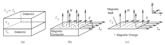
Figure \(\PageIndex{2}\): Properties of the EM field at a magnetic wall: (a) the interface of two dielectrics of contrasting permittivities approximates a magnetic wall with the magnetic field perpendicular to the interface and the electric field parallel to it; (b) the dielectric with lower permittivity can be approximated as a magnetic conductor; and (c) the magnetic conductor forms a magnetic wall at the interface with the material with higher permittivity.
| Electric field | Magnetic field | |
|---|---|---|
| Electric wall | Normal | Parallel |
| Magnetic wall | Parallel | Normal |
Table \(\PageIndex{1}\): Properties of electric and magnetic walls.
What constitutes a good magnetic wall is subject to debate, as the contrast between dielectrics is not as great as the contrast between the conductivity of a good conductor and that of a good dielectric. However, it is an essential concept in understanding the coupling of signals and approximating transmission lines to yield intuitive understanding.
The summary that is used in the text to understand multimoding is given in Table \(\PageIndex{1}\).