1.A: Appendix- Mathematical Foundations

1.A.1 Angles of a Triangle

The law of cosines relates the angles and lengths of the sides of the triangle in Figure \(\PageIndex{1}\)(a):

\[\begin{align}\label{eq:1}c^{2}&=a^{2}+b^{2}-2ab\cos(\gamma) \\ \label{eq:2} \cos(\alpha)=\frac{b^{2}+c^{2}-a^{2}}{2bc},\quad\cos(\beta)&=\frac{a^{2}+c^{2}-b^{2}}{2ac},\quad\cos(\gamma)=\frac{a^{2}+b^{2}-c^{2}}{2ab}\end{align} \]

Referring to the right-angle triangle in Figure \(\PageIndex{1}\)(b):

\[\label{eq:3}\sin(x)=\frac{\text{opposite}}{\text{hypotenuse}},\quad\cos(x)=\frac{\text{adjacent}}{\text{hypotenuse}},\quad\tan(x)=\frac{\text{opposite}}{\text{adjacent}} \]

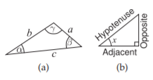
Figure \(\PageIndex{1}\): Triangles: (a) triangle with sides having lengths \(a, b,\) and \(c\), and angles \(\alpha, \beta,\) and \(\gamma\); and (b) right-angle triangle.

1.A.2 Trigonometric Identities

\[\begin{align}\label{eq:4}\text{if }\sin(\theta)&=x\text{ then }\theta =\arcsin(x)\quad\text{if}\quad\cos(\theta)=x\text{ then }\theta =\arccos(x)\\ \label{eq:5}\text{if }\tan(\theta)&=x\text{ then }\theta =\arctan(x)\end{align} \]

\[\begin{align} \label{eq:6}\sin(-x)&=-\sin x &\cos(-x)&=\cos(x) &\tan(-x)&=-\tan x\\ \label{eq:7}\csc(-x)&=-\csc x &\sec(-x)&=\sec x &\cot(-x)&=-\cos x\end{align} \]

\[\label{eq:8}\cos(x)=\frac{1}{2}(e^{\jmath x}+e^{-\jmath x})\qquad \sin(x)=\frac{1}{2}\jmath(e^{-\jmath x}-e^{\jmath x}) \]

\[\begin{align}\label{eq:9}\sin x&=1/\csc x &\cos x&=1/\sec x &\tan x&=1/\cot x\\ \label{eq:10}\tan x&=\sin x/\cos x\end{align} \]

\[\label{eq:11}\sin^{2}x+\cos^{2}x=1\qquad 1+\tan^{2}x=\sec^{2}x\qquad 1+\cot^{2}x=\csc^{2}x \]

\[\begin{align}\label{eq:12}\sin\left(x-\frac{\pi}{2}\right)&=-\cos x &\cos\left(x-\frac{\pi}{2}\right)&=\sin x &\tan\left(x-\frac{\pi}{2}\right)&=-\cot x\\ \label{eq:13}\sin\left(x+\frac{\pi}{2}\right)&=\cos x &\cos\left(x+\frac{\pi}{2}\right)&=-\sin x &\tan\left(x+\frac{\pi}{2}\right)&=-\cot x\\ \label{eq:14}\sin\left(\frac{\pi}{2}-x\right)&=\cos x &\cos\left(\frac{\pi}{2}-x\right)&=\sin x &\tan\left(\frac{\pi}{2}-x\right)&=\cot x \\ \label{eq:15} \csc\left(x-\frac{\pi}{2}\right)&=-\sec x &\sec\left(x-\frac{\pi}{2}\right)&=\csc x &\cot\left(x-\frac{\pi}{2}\right)&=-\tan x \\ \label{eq:16} \csc\left(x+\frac{\pi}{2}\right)&=\sec x &\sec\left(x+\frac{\pi}{2}\right)&=-\csc x &\cot\left(x+\frac{\pi}{2}\right)&=-\tan x \\ \label{eq:17}\csc\left(\frac{\pi}{2}-x\right)&=\sec x &\sec\left(\frac{\pi}{2}-x\right)&=\csc x &\cot\left(\frac{\pi}{2}-x\right)&=\tan x\end{align} \]

\[\begin{align}\label{eq:18}\sin (2x)&=2\sin x\cos y &\cos(2x)&=\cos^{2}(x)-\sin^{2}(x)\\ \label{eq:19}\tan (2x)&=\frac{2\tan x}{1-\tan^{2}x} &\cot (2x)&=\frac{1}{2}[\cot (x)-\tan (x)]\end{align} \]

\[\label{eq:20}\sin^{2}x=\frac{1}{2}[1-\cos (2x)]\qquad \cos^{2}x=\frac{1}{2}[1+\cos (2x)]\qquad \tan^{2}x=\frac{1-\cos (2x)}{1+\cos (2x)} \]

\[\begin{align} \label{eq:21} \tan (x+y)&=\frac{\tan(x)+\tan(y)}{\tan(x)-\tan(y)} &\tan(x-y)&=\frac{\tan(x)-\tan(y)}{\tan(x)+\tan(y)} \\ \label{eq:22} \sin x+\sin y&=2\sin\left(\frac{x+y}{2}\right)\cos\left(\frac{x-y}{2}\right) &\sin x-\sin y &=2\cos\left(\frac{x+y}{2}\right)\sin\left(\frac{x-y}{2}\right) \\ \label{eq:23} \cos x+\cos y&=2\cos\left(\frac{x+y}{2}\right)\cos\left(\frac{x-y}{2}\right) &\cos x-\cos y&=-2\cos\left(\frac{x+y}{2}\right)\sin\left(\frac{x-y}{2}\right)\end{align} \]

\[\begin{align}\label{eq:24}\sin x\sin y&=\frac{1}{2}[\cos (x-y)-\cos (x+y)] &\sin x\cos y&=\frac{1}{2}[\sin (x+y) +\sin (x-y)] \\ \label{eq:25}\cos x\cos y&=\frac{1}{2}[\cos (x-y)+\cos (x+y)] &\cos x\sin y&=\frac{1}{2}[\sin (x+y)-\sin (x-y)]\end{align} \]

1.A.3 Trigonometric Derivatives

\[\begin{align} \frac{d}{dx}\sin (x)&=\cos (x) &\frac{d}{dx}\cos (x)&=-\sin (x) &\frac{d}{dx}\tan (x)&=\sec^{2}(x) \nonumber\\ \frac{d}{dx}\csc (x)&=-\csc (x)\cot(x) &\frac{d}{dx}\sec (x)&=\sec (x)\tan (x) &\frac{d}{dx}\cot (x)&=-\csc^{2}(x)\nonumber\end{align} \nonumber \]

1.A.4 Complex Numbers and Phasors

A complex number \(z\) is an ordered pair of two real numbers \(x\) and \(y\), and a complex number has a special meaning when working in the frequency domain. The rectangular form of the complex number is \(z = x +\jmath y\), where \(\jmath =\sqrt{-1}\) is an imaginary number.\(^{1}\) The polar form of the complex number \(z = r\angle\varphi\) relates directly to the amplitude and phase of a cosinusoid. In determining phase, reference is made to a cosinusoid of the form \(u(t) = r \cos (\omega t +\varphi)\), as this has a value of \(r\) when the radian frequency \(\omega = 0\) (i.e., at DC). The cosinusoid is shown as the solid line in Figure \(\PageIndex{2}\)(a), where \(r\) is the amplitude and \(\phi\) is the phase of the cosinusoid. The cosinusoid can be presented as the complex valued function

\[\label{eq:27}f(t)=ze^{\jmath\omega t},\qquad\text{where}\qquad z=re^{\jmath\phi} \]

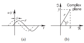
Figure \(\PageIndex{2}\): Sinusoidal signal representations: (a) waveform referenced to the zerophase cosinusoid shown as the dashed waveform; and (b) representation as a phasor on the complex plane where \(Re\) is the real part and \(Im\) is the imaginary part.

is called the phasor of \(u(t)\). The phasor contains the amplitude and phase of the cosinusoid, and given the frequency of the cosinusoid, the original time-domain waveform can be reconstructed. The time-domain form of the complex function is

\[\label{eq:28} u(t)=\Re\left\{f(t)\right\} =\Re\left\{ze^{\jmath\omega t}\right\}=\Re\left\{re^{\jmath\phi}e^{\jmath\omega t}\right\}=\Re\left\{re^{[\jmath (\omega t+\phi)]}\right\}=r\cos(\omega t+\phi) \]

\(\Re\{\:\:\}\) indicates that the real part of a complex number is taken, and similarly \(\Im\{\:\:\}\) indicates that the imaginary part of a complex number is taken. The complex number can be represented in rectangular or magnitude-phase form so that

\[\label{eq:29}z=x+\jmath y=r\angle\phi =re^{\jmath\phi}=r(\cos\phi +\jmath\sin\phi) \]

with the relationship shown in Figure \(\PageIndex{2}\)(b). Note that in Equation \(\eqref{eq:29}\), \(\phi\) must be expressed in radians and anywhere it is used in calculations. Also

\[\label{eq:30}x=r\cos(\phi)\quad\text{and}\quad y=r\sin(\phi) \]

Basic calculations using the complex numbers

\[\label{eq:31}w=a+\jmath b=q\angle\theta\quad\text{and}\quad z=c+\jmath d=r\angle \phi \]

(with \(a,\: b,\: c,\: d ,\:\theta ,\:\phi ,\: r\), and \(q\) being real numbers) are

• \(\jmath\cdot\jmath=\jmath^{2}=-1\)
• Addition: \(w + z = (a +\jmath b)+(c +\jmath d)=(a + c) + \jmath (b + d)\)
• Subtraction: \(w − z = (a + \jmath b) − (c + \jmath d)=(a − c) + \jmath (b − d)\)
• Multiplication: \(w\cdot z = (a + \jmath b) \cdot (c +\jmath d)=(ac − bd) + \jmath (bc + ad)\)
• Magnitude: \(|w| = \sqrt{a^{2} + b^{2}} = q;\: |z| = \sqrt{c^{2} + d^{2}} = r\)
• Angle: \(\theta = \arctan(b/a) = \arccos(a/q) = \arcsin(b/q)\) (Correction may be required to get the phase in the right quadrant. This requires that the signs of a and b be examined.)
• Multiplication (alternative): \(w\cdot z = qr\angle (\theta +\phi )\)
• Division: \(w/z = \frac{a +\jmath b}{c +\jmath d} = \frac{(a + \jmath b)(c − \jmath d)}{(c + \jmath d)(c −\jmath d)} =\left(\frac{ac + bd }{c^{2} + d^{2}}\right) +\jmath\left(\frac{bc − ad}{c^{2} + d^{2}}\right)\)
• Division (alternative): \(w/z = q/r\angle (\theta − \phi)\)
• Square root: \(\sqrt{w} = \sqrt{q}\angle (\theta /2+m\pi ),\:\: m = 0, 1\) (i.e. \(\sqrt{w} = \sqrt{q}\angle (\theta /2)\) and \(\sqrt{q}\angle (\theta /2+\pi )\))
• \(n\)th root: \(\sqrt[n]{w} = \sqrt[n]{q}\angle \left(\theta /n + 2\pi\frac{m}{n}\right) ,\:\: m = 0, 1,\ldots (n − 1)\)
• Negative: \(−w = −q\angle\theta = q\angle (\theta + \pi )\)
• Complex conjugate: \(w^{\ast} = a −\jmath b = q\angle (−\theta )\)
• Squared magnitude: \(|z|^{2} = z\cdot z^{\ast}\)
• Conjugate addition: \((w + z)^{\ast} = w^{\ast} + z^{\ast}\)
• Conjugate power: \((z^{n})^{\ast} = (z^{\ast})^{n}\)
• Conjugate multiplication: \((wz)^{\ast} = w^{\ast}z^{\ast}\)
• Conjugate division: \((w/z)^{\ast} = w^{\ast}/z^{\ast}\)
• Conjugate exponential: \(\exp(z^{\ast}) = (\exp z)^{\ast}\)
• Conjugate logarithm: \(\log(z^{\ast}) = (\log z)^{\ast}\)
• Conjugate conjugate: \((w^{\ast})^{\ast} = w\)
• Complex inverse: \(z^{−1} = z^{\ast}/|z|^{2}\)
• Complex magnitude: \(|z^{\ast}| = |z|\)

Example \(\PageIndex{1}\): Complex numbers

Consider the complex numbers \(w = −0.5 −\jmath 1.6\) and \(z = 5 −\jmath 3\), and the waveform \(v(t)=2.3 \cos(2\pi 10t − 1.2)\).

• In polar form, \(w = 1.676\angle (−1.874)\), where \(1.874\) is in radians; alternatively \(w = 1.676\angle (−107.4)^{\circ}\).
• In polar form, \(z = 5.831\angle (−0.54)\).
• \(2w = −1 − \jmath 3.2 = 3.353\angle (−1.874)\).
• \(z\cdot w = w\cdot z = w\cdot z = (1.676\cdot 5.831)\angle (−1.874−0.54) = 9.774\angle (−2.414) = −7.3−\jmath 6.5\).
• \(\sqrt{z} = 2.327 −\jmath 0.645\).
• Alternatively \(\sqrt{z} = \sqrt{5.831}\angle (−0.54/2)=2.415\angle (−0.27)\).
• \(w/z = (1.676/5.831)\angle [−1.874 − (−0.54)] = 0.287\angle −1.333 = 0.068 −\jmath 6.5\).
• The radian frequency of \(v(t)\) is \(20\pi\text{ rads/s}\).
• The frequency of \(v(t)\) is \(10\text{ Hz}\).
• The phasor of \(v(t)\) is \(v = 2.3\angle (−1.2) = 2.3\angle (−68.755^{\circ})=0.833 −\jmath 2.144\).
• If \(w\) is a phasor and its frequency is \(1\text{ GHz}\), the waveform equivalent of \(w\) is \(w(t) = 1.676 \cos(2\pi\cdot 10^{9}t − 1.874)\) and the phase is \(−1.874\) radians or \(−107.35^{\circ}\) or \(252.65^{\circ}\).

1.A.5 Vector Operators

Vector Multiplication

There are two types of operations that multiply vectors. \(\mathbf{A},\: \mathbf{B},\) and \(\mathbf{C}\) are vectors with

\[\label{eq:32}\mathbf{A}=a_{i}\mathbf{i}+a_{j}\mathbf{j}+a_{k}\mathbf{k} \]

where \(\mathbf{i},\: \mathbf{j},\) and \(\mathbf{k}\), are orthogonal vectors such as the unit vectors of the Cartesian coordinate system, that is, \(\hat{\mathbf{x}},\: \hat{\mathbf{y}},\) and \(\hat{\mathbf{z}}\) in the \(x,\: y,\) and \(z\) directions, respectively

Dot Product

\(\mathbf{A}\cdot\mathbf{B}\) is called the dot product, the scalar product or the inner product. It is read as “a dot b.”

\(\mathbf{A}\cdot\mathbf{B}=a_{i}b_{i}+a_{j}b_{j}+\ldots +a_{k}b_{k}\)

Commutative property: \(\mathbf{A}\cdot\mathbf{B} = \mathbf{B}\cdot\mathbf{A}\).

Distributive property: \(\mathbf{A}\cdot (\mathbf{B} +\mathbf{C}) = \mathbf{A}\cdot\mathbf{B} + \mathbf{A}\cdot\mathbf{C}\).

Bilinear property (\(r\) is a scalar): \(\mathbf{A}\cdot (r\mathbf{B} + \mathbf{C}) = r(\mathbf{A}\cdot\mathbf{B})+(\mathbf{A}\cdot\mathbf{C})\).

Scalar multiplication property (\(r\) and \(s\) are scalars): \((r\mathbf{A})\cdot (s\mathbf{B})=(rs)(\mathbf{A}\cdot\mathbf{B})\).

Orthogonal property: Two nonzero vectors \(\mathbf{A}\) and \(\mathbf{B}\) are orthogonal if and only if \(\mathbf{A}\cdot\mathbf{B} = 0\).

Cross Product

\(\mathbf{A}\times\mathbf{B}\) is called the cross product. It is read as “a cross b.” Now the vector components of \(\mathbf{A},\: \mathbf{B},\) and \(\mathbf{C}\) need to be more tightly specified as orthogonal vectors, typically having unit amplitude, that have the property

\[\begin{align}\label{eq:33}\mathbf{i}\times\mathbf{j}&=\mathbf{k} &\mathbf{j}\times\mathbf{k}&=\mathbf{i} &\mathbf{k}\cdot\mathbf{i}&=\mathbf{j},\quad\text{and} &\mathbf{i}\times\mathbf{i}&=0=\mathbf{j}\times\mathbf{j}=\mathbf{k}\times\mathbf{k} \\ \label{eq:34} \mathbf{j}\times\mathbf{i}&=-\mathbf{k} &\mathbf{k}\times\mathbf{j}&=-\mathbf{i} &\mathbf{i}\times\mathbf{k}&=-\mathbf{j}\end{align} \]

The unit vectors of the Cartesian coordinate system have this property with \(\mathbf{i},\: \mathbf{j},\) and \(\mathbf{k}\), corresponding to the unit vectors \(\hat{\mathbf{x}}\), \(\hat{\mathbf{y}}\), and \(\hat{\mathbf{z}}\) in the \(x,\: y,\) and \(z\) directions, respectively.

\[\begin{align}\mathbf{a}\times\mathbf{b}&=(a_{i}\mathbf{i}+a_{j}\mathbf{j}+a_{k}\mathbf{k})\times (b_{i}\mathbf{i}+b_{j}\mathbf{j}+b_{k}\mathbf{k})\nonumber \\ &=a_{i}b_{i}\mathbf{i}\times\mathbf{i}+a_{i}b_{j}\mathbf{i}\times\mathbf{j}+a_{i}b_{k}\mathbf{i}\times\mathbf{k}+a_{j}b_{i}\mathbf{j}\times\mathbf{i}+a_{j}b_{j}\mathbf{j}\times\mathbf{j}+a_{j}b_{k}\mathbf{j}\times\mathbf{k} +\nonumber \\ &\quad a_{k}b_{i}\mathbf{k}\times\mathbf{i}+a_{k}b_{j}\mathbf{k}\times\mathbf{j}+a_{k}b_{k}\mathbf{k}\times\mathbf{k}\nonumber \\ \label{eq:35} &=(a_{j}b_{k}-a_{k}b_{j})\mathbf{i}+(a_{k}b_{i}-a_{i}b_{k})\mathbf{j}+(a_{i}b_{j}-a_{j}b_{i})\mathbf{k}\end{align} \]

Anticommutative property: \(\mathbf{A}\times\mathbf{B} = −\mathbf{B}\times\mathbf{A}\).

Distributive property: \(\mathbf{A}\times (\mathbf{B} +\mathbf{C}) = \mathbf{A}\times \mathbf{B} + \mathbf{A}\times\mathbf{C}\).

Bilinear property (\(r\) is a scalar): \(\mathbf{A}\times (r\mathbf{B} + \mathbf{C}) = r(\mathbf{A}\times \mathbf{B})+(\mathbf{A}\times \mathbf{C})\).

Scalar multiplication property (\(r\) and \(s\) are scalars): \((r\mathbf{A})\times (s\mathbf{B})=(rs)(\mathbf{A}\times\mathbf{B})\).

Lagrange's formula

\(\mathbf{A}\times (\mathbf{B}\times\mathbf{C})=\mathbf{B}(\mathbf{B}\cdot\mathbf{C})-\mathbf{C}(\mathbf{A}\cdot\mathbf{B})\)

Del (\(\nabla\)) Vector Operator

Operations in Cartesian, Cylindrical, and Spherical Coordinate Systems

This section defines the del, or the nabla \(\nabla\), a calculus operator that operates on vector quantities and also on a scalar to create a vector. The various del operators in the Cartesian (rectangular), spherical, and cylindrical coordinate systems are presented. Here a scalar is denoted by \(f\) and a vector by \(\mathbf{F}\):

• grad, \(\nabla\), is the gradient of a scalar with direction. \(\nabla f\) is read as “grad f.”
• div, \(\nabla\), is a measure of how a vector is spreading out from a point. \(\nabla\cdot\mathbf{F}\) is read as “div F.”
• curl, \(\nabla\times\), is a measure of the rotation of a vector. \(\nabla\times\mathbf{F}\) is read as “curl F.”

Cartesian (rectangular) coordinates \((x, y, z)\):

\(\hat{x}\) is the unit vector in the \(x\) direction and \(F_{x}\) is the component of the field in the \(x\)-direction. Similarly for the other components.

Figure \(\PageIndex{3}\)

\[\begin{align}\label{eq:36}\mathbf{F}&=F_{x}\hat{x}+F_{y}\hat{y}+F_{z}\hat{z} \\ \label{eq:37}\text{grad}\quad\nabla f&=\frac{\partial f}{\partial x}\hat{\mathbf{x}}+\frac{\partial f}{\partial y}\hat{\mathbf{y}}+\frac{\partial f}{\partial z}\hat{\mathbf{z}} \\ \label{eq:38}\text{div}\quad\nabla\cdot\mathbf{F}&=\frac{\partial F_{x}}{\partial x}+\frac{\partial F_{y}}{\partial y}+\frac{\partial F_{z}}{\partial z} \\ \label{eq:39}\text{curl}\quad\nabla\times\mathbf{F}&=\left(\frac{\partial F_{z}}{\partial y}-\frac{\partial F_{y}}{\partial z}\right)\hat{\mathbf{z}}+\left(\frac{\partial F_{x}}{\partial z}-\frac{\partial F_{z}}{\partial x}\right)\hat{\mathbf{y}}+\left(\frac{\partial F_{y}}{\partial x}-\frac{\partial F_{x}}{\partial y}\right)\hat{\mathbf{z}} \\ \label{eq:40}\nabla^{2}\mathbf{F}&=\frac{\partial^{2}\mathbf{F}}{\partial x^{2}}+\frac{\partial^{2}\mathbf{F}}{\partial y^{2}}+\frac{\partial^{2}\mathbf{F}}{\partial z^{2}} \\ \label{eq:41}\text{differential length, }d\ell &=dx\:\hat{\mathbf{x}}+dy\:\hat{\mathbf{y}}+dz\:\hat{\mathbf{z}} \\ \label{eq:42} \text{differential normal area, }d\mathbf{s}&=dy\:dz\:\hat{\mathbf{x}}+dx\:dz\:\hat{\mathbf{y}}+dx\:dy\:\hat{\mathbf{z}} \\ \label{eq:43} \text{differential volume, }dv&=dx\:dy\:dz\end{align} \]

Cylindrical coordinates \((\rho, \phi, z)\):

The cylindrical coordinates are \(\rho\) for radius, \(\phi\) for angle, and \(z\) for height. These are related to the Cartesian coordinates by

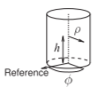
Figure \(\PageIndex{4}\)

\[\begin{align} \label{eq:44} x&=\rho\cos\phi,&y&=\rho\sin\phi, \quad z=z \\ \label{eq:45}\rho&=\sqrt{x^{2}+y^{2}} &\phi &=\text{atan}2(y,x), \quad z=z \\ \label{eq:46} &\text{vector} &\mathbf{F}&=F_{\rho}\hat{\mathbf{ρ}}+F_{\phi}\hat{\mathbf{ϕ}}+F_{z}\hat{\mathbf{z}} \\ \label{eq:47} &\text{grad} &\nabla f&=\frac{\partial f}{\partial\rho}\hat{\mathbf{ρ}} +\frac{1}{\rho}\frac{\partial f}{\partial\phi}\hat{\mathbf{ϕ}}+\frac{\partial f}{\partial z}\hat{\mathbf{z}} \\ \label{eq:48} &\text{div} &\nabla\cdot\mathbf{F}&=\frac{1}{\rho}\frac{\partial_{\rho}F_{\rho}}{\partial\rho} +\frac{1}{\rho}\frac{\partial F_{\phi}}{\partial\phi}+\frac{\partial F_{z}}{\partial z} \\ \label{eq:49} &\text{curl}&\nabla\times\mathbf{F}&=\left(\frac{1}{\rho}\frac{\partial F_{z}}{\partial\phi}-\frac{\partial F_{\phi}}{\partial z}\right)\hat{\mathbf{ρ}}+\left(\frac{\partial F_{\rho}}{\partial z}-\frac{\partial F_{z}}{\partial\rho}\right)\hat{\mathbf{ϕ}}+\frac{1}{\rho}\left(\frac{\partial (\rho F_{\phi})}{\partial\rho}-\frac{\partial F_{\rho}}{\partial\phi}\right)\hat{\mathbf{z}} \end{align} \]

\[\begin{align}\label{eq:50}\text{ differential length, }d\ell&=d\rho\hat{\mathbf{ρ}}+\rho \:d\phi \hat{\mathbf{ϕ}}+dz\:\hat{\mathbf{z}} \\ \label{eq:51}\text{differential normal area, }d\mathbf{s}&=\rho\: d\phi\: dz\hat{\mathbf{ρ}}+d\rho \:dz\:\hat{\mathbf{ϕ}}+\rho\:d\rho \:d\phi \hat{\mathbf{z}} \\ \label{eq:52}\text{differental volume, }dv&=\rho\: d\rho \:d\phi \:dz\end{align} \]

Spherical coordinates \((\rho, \theta, \phi)\):

The spherical coordinates are \(\rho\) for radius, \(\theta\) for angle of the horizontal projection, and \(\phi\) for the elevation angle. These are related to the Cartesian coordinates by

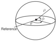
Figure \(\PageIndex{5}\)

\[\begin{align}\label{eq:53} x& =r\sin \theta \cos \phi , & y & =r\sin \theta \sin \phi, \quad z=r\cos \theta \\ \label{eq:54} r&=\sqrt{x^{2}+y^{2}+z^{2}} &\theta&=\arccos(z/r),\quad \phi=\text{atan}2(y, x) \\ \label{eq:55} &\text{vector} &\mathbf{F}&=F_{r}\hat{\mathbf{r}}+F_{\theta}\hat{\mathbf{θ}}+F_{\phi}\hat{\mathbf{ϕ}} \\ \label{eq:56} &\text{grad} &\nabla f&=\frac{\partial f}{\partial r}\hat{\mathbf{r}}+\frac{1}{r}\frac{\partial f}{\partial \theta}\hat{\mathbf{θ}}+\frac{1}{r\sin\theta}\frac{\partial f}{\partial\phi}\hat{\mathbf{ϕ}} \\ \label{eq:57}&\text{div}&\nabla\cdot\mathbf{F}&=\frac{1}{r^{2}}\frac{\partial (r^{2}F_{r})}{\partial r}+\frac{1}{r\sin\theta}\frac{\partial (F_{\theta}\sin\theta)}{\partial\theta}+\frac{1}{r\sin\theta}\frac{\partial F_{\phi}}{\partial\phi} \\ &\text{curl}&\nabla\times\mathbf{F}&=\frac{1}{r\sin\theta}\left(\frac{\partial(F_{\phi}\sin\theta)}{\partial\theta}-\frac{\partial F_{\theta}}{\partial\phi}\right)\hat{\mathbf{r}} \\ \label{eq:58}&&&\quad +\frac{1}{r}\left(\frac{1}{\sin\theta}\frac{\partial F_{r}}{\partial\theta}-\frac{\partial (rF_{\phi})}{\partial r}\right)\hat{\mathbf{θ}} +\frac{1}{r}\left(\frac{\partial (rF_{\theta})}{\partial r}-\frac{\partial F_{r}}{\partial\theta}\right)\hat{\mathbf{ϕ}} \end{align} \]

\[\begin{align}\label{eq:59}\text{differential length }d\ell &=dr\:\hat{\mathbf{r}}+r\:d\theta\:\hat{\mathbf{θ}} +r\sin\theta\:d\phi\:\hat{\mathbf{ϕ}} \\ \label{eq:60}\text{differential area }d\mathbf{s}&=r^{2}\sin\theta\:d\theta\:d\phi\:\hat{\mathbf{r}}+r\sin\theta\:dr\:d\phi\:\hat{\mathbf{θ}} +r\:dr\:d\theta\:\hat{\mathbf{ϕ}} \\ \label{eq:61}\text{differential volume }dv&=r^{2}\sin\theta\:dr\:d\theta\:d\phi\end{align} \]

Identities

Identities for the del, \(\nabla\), operator:

\[\begin{align}\label{eq:62}\text{div grad }f&=\nabla\cdot (\nabla f)=\nabla^{2}f=\Delta f\text{(Laplacian)} \\ \label{eq:63}\Delta (fg)&=f\Delta g+2\nabla f\cdot\nabla g+g\Delta f \\ \label{eq:64} \text{curl grad }f&=\nabla\times (\nabla f)=0 \\ \label{eq:65}\text{div curl }\mathbf{F}&=\nabla\cdot (\nabla\times\mathbf{F})=0 \\ \label{eq:66}\text{curl curl }\mathbf{F}&=\nabla\times (\nabla\times\mathbf{F})=\nabla (\nabla\cdot F)-\nabla^{2}F \\ \label{eq:67}\mathbf{A}\times (\mathbf{B}\times\mathbf{C})&=\mathbf{B}(\mathbf{A}\cdot\mathbf{C})-\mathbf{C}(\mathbf{A}\cdot\mathbf{B})\end{align} \]

1.A.6 Hyperbolic Functions and Complex Numbers

\[\begin{align}\label{eq:68}\cosh (x)&=\frac{1}{2}(e^{x}+e^{-x})=\cos (\jmath x) \\ \label{eq:69}\cosh (\jmath x)&=\frac{1}{2}(e^{\jmath x}+e^{-\jmath x})=\cos (x) \\ \label{eq:70}\cosh (-x)&=\cosh (x)\end{align} \]

\[\begin{align}\label{eq:71}\sinh(x)&=\frac{1}{2}(e^{x}-e^{-x})=-\jmath\sin(\jmath x) \\ \label{eq:72}\sinh (\jmath x)&=\frac{1}{2}(e^{\jmath x}-e^{-\jmath x})=\jmath\sin (x) \\ \label{eq:73}\sinh(-x)&=-\sinh (x)\end{align} \]

\[\label{eq:74}\cosh^{2}(x)-\sinh^{2}(x)=1 \]

\[\begin{align}\label{eq:75}\tanh(x)&=\sinh(x)/\cosh(x) \\ \label{eq:76}\tanh(x)&=-\jmath\tan(\jmath x) \\ \label{eq:77}\tanh(\jmath x)&=\jmath\tan(x) \\ \label{eq:78} \tanh(-x)&=-\tanh(x)\end{align} \]

\[\begin{align}\label{eq:79}\sin(\jmath x)&=\jmath\sinh(x) \\ \label{eq:80}\cos(\jmath x)&=\cosh (x) \\ \label{eq:81}\tan(\jmath x)&=\jmath\tanh(x)\end{align} \]

\[\begin{align}\label{eq:82}e^{x}&=\cosh(x)+\sinh(x) &e^{-x}&=\cosh(x)-\sinh(x) \\ \label{eq:83}e^{\jmath x}&=\cos(x)+\jmath\sin(x) &e^{-\jmath x}&=\cos(x)-\jmath\sin(x)\end{align} \]

\[\begin{align}\label{eq:84}\sin(x+\jmath y)&=\sin(x)\cosh(y)+\jmath\cos(x)\sinh(y) \\ \label{eq:85}\cos(x+\jmath y)&=\cos(x)\cosh(y)-\jmath\sin(x)\sinh(y)\end{align} \]

\[\label{eq:86}e^{\gamma}=e^{(\alpha +\jmath\beta)}=e^{\alpha}e^{\jmath\beta},\text{ where }\gamma =\alpha +\jmath\beta \]

\[\label{eq:87}\cot(x)=\frac{1}{2}[\cot (x/2)-\tan(x/2)] \]

1.A.7 Volumes and Areas

	Circle	Sphere	Cylinder	Cone
	\(r=\) radius	\(r=\) radius	\(r=\) radius \(h=\) height	\(r=\) radius of base \(h=\) height
Area	\(\pi r^{2}\)	\(4\pi r^{2}\)	\(2\pi rh\) (cylinder) \(2\pi r^{2}\) (base & top)
Volume		\(4\pi r^{3}/3\)	\(\pi r^{2}h\)	\(\pi r^{2}h/3\)

Table \(\PageIndex{1}\)

1.A.8 Series Expansions

Square root:

\[\begin{align} \sqrt{1+x}&=\sum_{n=0}^{\infty}\frac{(-1)^{n}(2n)!}{(1-2n)(n!)^{2}(4^{n})}x^{n}\nonumber \\ \label{eq:88}&=1+\frac{1}{2}x-\frac{1}{8}x^{2}+\frac{1}{16}x^{3}-\frac{5}{128}x^{4}+\ldots \text{ for }-1< x\leq 1\end{align} \]

Exponential function (the natural number e raised to a power):

\[\label{eq:89}e^{x}=\sum_{n=0}^{\infty}\frac{x^{n}}{n!}=1+x+\frac{x^{2}}{2!}+\frac{x^{3}}{3!}+\ldots\text{ for all }x \]

Natural logarithm:

\[\begin{align} \label{eq:90}\ln(1-x)&=-\sum_{n=1}^{\infty}\frac{x^{n}}{n}\text{ for }-1\leq x<1 \\ \label{eq:91}\ln(1+x)&=\sum_{n=1}^{\infty}(-1)^{n+1}\frac{x^{n}}{n}\text{ for }-1<x\leq 1\end{align} \]

Binomial series:

\[\label{eq:92}(1+x)^{\alpha}=\sum_{n=0}^{\infty}\left(\begin{array}{c}{\alpha}\\{n}\end{array}\right)x^{n}\quad\text{ for all }|x|<1\text{ and all complex }\alpha \]

where \(n\) is an integer and the binomial coefficient is

\[\label{eq:93} \left(\begin{array}{c}{\alpha}\\{n}\end{array}\right)=\prod_{k=1}^{n}\frac{\alpha -k+1}{k}=\frac{\alpha (\alpha -1)\ldots (\alpha -n+1}{n!} \]

If \(\alpha\) is replaced by an integer \(N\) the binomial coefficient is

\[\label{eq:94} \left(\begin{array}{c}{N}\\{n}\end{array}\right)=\frac{N!}{(N-n)!n!} \]

Infinite geometric series:

\[\begin{align}\label{eq:95}\frac{1}{1-x}&=\sum_{n=0}^{\infty}x^{n}\quad\text{for }|x|<1 \\ \label{eq:96}\frac{x}{(1-x)^{2}}&=\sum_{n=1}^{\infty}nx^{n}\quad\text{for }|x|<1 \\ \label{eq:97}\frac{1}{(1-x)^{2}}&=\sum_{n=1}^{\infty}nx^{n-1}\quad\text{for }|x|<1\end{align} \]

1.A.9 Trigonometric Series Expansions

\[\begin{align}\label{eq:98} \sin x&=\sum_{n=0}^{\infty}\frac{(-1)^{n}}{(2n+1)!}x^{2n+1}=x-\frac{x^{3}}{3!}+\frac{x^{5}}{5!}-\cdots\text{ for all }x \\ \label{eq:99} \cos x&=\sum_{n=0}^{\infty}\frac{(-1)^{n}}{(2n)!}x^{2n}=1-\frac{x^{2}}{2!}+\frac{x^{4}}{4!}-\cdots\text{ for all }x \\ \label{eq:100}\tan x&=x+\frac{x^{3}}{3}+\frac{2x^{5}}{15}+\cdots\text{ for }|x|<\frac{\pi}{2} \\ \label{eq:101}\sinh x&=\sum_{n=0}^{\infty}\frac{x^{2n+1}}{(2n+1)!}=x+\frac{x^{3}}{3!}+\frac{x^{5}}{5!}+\cdots\text{ for all }x \\ \label{eq:102} \cosh x&=\sum_{n=0}^{\infty}\frac{x^{2n}}{(2n)!}=1+\frac{x^{2}}{2!}+\frac{x^{4}}{4!}+\cdots\text{ for all }x \\ \label{eq:103}\tanh x&=\sum_{n=1}^{\infty}\frac{B_{2n}4^{n}(4^{n}-1)}{(2n)!}x^{2n-1}=x-\frac{1}{3}x^{3}+\frac{2}{15}x^{5}-\frac{17}{315}x^{7}+\cdots\text{ for }|x|<\frac{\pi}{2} \\ \label{eq:104}\text{arsinh}(x)&=\sum_{n=0}^{\infty}\frac{(-1)^{n}(2n)!}{4^{n}(n!)^{2}(2n+1)}x^{2n+1}\text{ for }|x|\leq 1 \\ \label{eq:105} \text{artanh}(x)&=\sum_{n=0}^{\infty}\frac{x^{2n+1}}{2n+1}\text{ for }|x|<1\end{align} \]

1.A.10 Special Polynomials

Several polynomials have special properties of use in the design of filters and matching networks. Their arguments are put in terms of frequency and a transfer function of a two-port is expressed in terms on one of the special polynomials or its inverse.

Butterworth Polynomial

The Butterworth polynomials have the general form

\[\label{eq:106}B_{n}(x)=\left\{\begin{array}{ll}{\prod_{k=1}^{n/2}\left\{x^{2}-2x\cos\left[\frac{(2k+n-1)\pi}{2n}\right]+1\right\}}&{\text{for }n\text{ even}}\\{(x+1)\prod_{k=1}^{(n-1)/2}\left\{x^{2}-2x\cos\left[\frac{(2k+n-1)\pi}{2n}\right]+1\right\}}&{\text{for }n\text{ odd}}\end{array}\right. \]

These of course do not look like polynomials but their expansions are, see Table \(\PageIndex{2}\).

Chebyshev Polynomial

The \(n\)th-order Chebyshev polynomial of the first kind, \(T_{n}(x)\), (often just called the Chebyshev polynomial) has the special property that the maximum absolute value of \(T_{n}(x)\) for \(−1\leq x\leq 1\) is \(1\). This can be seen in the figure to the right where the first four Tchebyshev polynomials are plotted.

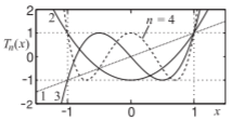
Figure \(\PageIndex{6}\)

When \(x\) is frequency this means that the frequency response in a bandwidth has equal ripples across the passband and outside (both above and below) the value of \(T_{n}(x)\) rapidly diverges (the magnitude becomes monotonically larger). For a filter or matching network the reflection coefficient is expressed in terms of \(T_{n}(x)\) and so the skirts of the transmission response are steep. Normalization of \(x\) and scaling of the Chebyshev polynomials is used to scale the response in frequency and amplitude. The Chebyshev polynomial is obtained using the recursion formula

\[\label{eq:107}T_{n}(x)=2xT_{n-1}-T_{n-2}(x)\quad\text{with}\quad T_{1}(x)=x\quad\text{and}\quad T_{2}(x)=2x^{2}-1 \]

For example, with \(n = 3\),

\[\label{eq:108}T_{3}(x)=2xT_{3-1}(x)-T_{3-2}(x)=2x(2x^{2}-1)-x=4x^{3}-2x-x=4x^{3}-3x \]

\(n\)	Butterworth Polynomial \(B_{n}(x)\)
\(1\)	\(x+1\)
\(2\)	\(x^{2}+1.4142x+1\)
\(3\)	\((x+1)(x^{2}+x+1\)
\(4\)	\((x^{2} + 0.7564x + 1)(x^{2} + 1.8478x + 1)\)
\(5\)	\((x + 1)(x^{2} + 0.1680x + 1)(x^{2} + 1.6180x + 1)\)
\(6\)	\((x^{2} + 0.5176x + 1)(x^{2} + 1.4142x + 1)(x^{2} + 1.9319x + 1)\)
\(7\)	\((x + 1)(x^{2} + 0.4450x + 1)(x^{2} + 1.2470x + 1)(x^{2} + 1.8019x + 1)\)
\(8\)	\((x^{2} + 0.3902x + 1)(x^{2} + 1.1111x + 1)(x^{2} + 1.6629x + 1)(x^{2} + 1.9616x + 1)\)

Table \(\PageIndex{2}\): Butterworth polynomials.

Several useful expansions of Chebyshev polynomials are used in microwave engineering to relate the frequency response of a function or circuit to the Chebyshev characteristic. Generally the frequency is referred to the electrical length \(\theta\) (which for a transmission line \(\theta\) is proportional to frequency). Some of the more useful expansions used in the text follow:

\[\label{eq:109}T_{n}(\cos\theta)=\cos(n\theta) \]

and note that when \(\theta = \pi /2, \cos(n\theta )=0\) when is odd and \(\cos(n\theta ) = \pm 1\) when is even. From this identity two more useful identities are derived:

\[\label{eq:110}T_{n}(x) = \cos\left( n \cos^{−1} x\right)\quad\text{for}\quad |x| ≤ 1,\quad\text{and}\quad T_{n}(x) = \cosh\left( n \cosh^{−1} x\right)\quad\text{for}\quad |x| ≥ 1 \]

A normalized argument \(\cos\theta/ \cos\theta_{m}\) is often used to define a passband as being between \(\theta_{m}\) and \((\pi −\theta_{m})\). That is that we can relate the Chebyshev response to frequency and define a frequency bandwidth. Then a useful Chebyshev polynomial expansion is

\[\label{eq:111} T_{n} (\cos\theta /\cos\theta_{m}) = T_{n}(\sec\theta_{m}\cos\theta) = \cos\left\{ n\left[ \cos^{−1} (\cos\theta/\cos\theta_{m})\right]\right\} \]

From Section 1.A.2 note that \(\cos^{2}\theta = \frac{1}{2} [1 + \cos(2\theta)]\), \(\cos\theta \cos(n\theta) = \frac{1}{2} \cos[(n + 1)\theta] \cos[(n − 1)\theta]\), and \(\sec(\theta_{m})=1/ \cos\theta_{m}\). Then (after ingenious manipulation) Equation \(\eqref{eq:107}\) becomes

\[\begin{align}T_{1}(\cos\theta /\cos\theta_{m})&=\sec\theta_{m}\cos\theta \nonumber \\ T_{2}(\cos\theta/\cos\theta_{m})&=\sec^{2}\theta_{m}[\cos(2\theta)+1]-1=\sec^{2}\theta_{m}\cos(2\theta)+(\sec^{2}\theta_{m}-1) \nonumber \\ T_{3}(\cos\theta/\cos\theta_{m})&=\sec^{3}\theta_{m}[\cos(3\theta)+3\cos\theta]-3\sec\theta_{m}\cos\theta \nonumber \\ &=\sec^{3}\theta_{m}\cos(3\theta)+3(\sec^{3}\theta_{m}-\sec\theta_{m})\cos\theta\nonumber \\ T_{4}(\cos\theta/\cos\theta_{m})&=\sec^{4}\theta_{m}[\cos(4\theta)+4\cos(2\theta)+3]-4\sec^{2}\theta_{m}[\cos(2\theta)+1]+1\nonumber \\ &=\sec^{4}\theta_{m}\cos(4\theta)+4(\sec^{4}-\sec^{2}\theta_{m})\cos(2\theta)+(3\sec^{4}\theta_{m}-4\sec^{2}\theta_{m}+1)\nonumber \\ K_{5}(\cos\theta/\cos\theta_{m})&=\sec^{5}\theta_{m}[\cos(5\theta)+5\cos(3\theta)+7\cos\theta]-\sec^{3}\theta_{m}[5\cos(3\theta)+11\cos\theta] \nonumber \\ &\quad +4\sec\theta_{m}\cos\theta\nonumber \\ &=\sec^{5}\theta_{m}\cos(5\theta)+5(\sec^{5}\theta_{m}-\sec^{3}\theta_{m})\cos(3\theta)\nonumber \\ \label{eq:112}&\quad +(7\sec^{5}\theta_{m}-11\sec^{3}\theta_{m}+4\sec\theta_{m})\cos\theta\end{align} \]

1.A.11 Matrix Operations

\(\mathbf{A}\), \(\mathbf{B}\), and \(\mathbf{C}\) are square matrices and V is a vector.

Determinant:

\[\label{eq:113}|\mathbf{A}|=\det (\mathbf{A}) \]

Transpose:

\[\begin{align}\label{eq:114}(\mathbf{ABC})^{\text{T}}&=\mathbf{C}^{\text{T}}\mathbf{B}^{\text{T}}\mathbf{A}^{\text{T}} \\ \label{eq:115}(\mathbf{ABC}^{\text{T}})^{\text{T}}&=\mathbf{CB}^{\text{T}}\mathbf{A}^{\text{T}}\end{align} \]

Inverse:

\[\begin{align}\label{eq:116}(\mathbf{ABC})^{-1}&=\mathbf{C}^{-1}\mathbf{B}^{-1}\mathbf{A}^{-1} \\ \label{eq:117}(\mathbf{ABC}^{-1})^{-1}&=(\mathbf{C}^{-1})^{-1}\mathbf{B}^{-1}\mathbf{A}^{-1}=\mathbf{CB}^{-1}\mathbf{A}^{-1} \\ \label{eq:118}\mathbf{AA}^{-1}&=\mathbf{A}^{-1}\mathbf{A}=\mathbf{I}=\mathbf{1}\end{align} \]

Two row square matrices and vectors

\[\label{eq:119}\mathbf{A} = \left[\begin{array}{cc}{a_{11}}&{a_{12}}\\{a_{21}}&{a_{22}}\end{array}\right]\quad\mathbf{B}=\left[\begin{array}{cc}{b_{11}}&{b_{12}}\\{b_{21}}&{b_{22}}\end{array}\right]\quad\mathbf{V}=\left[\begin{array}{c}{v_{1}}\\{v_{2}}\end{array}\right] \]

Multiplication:

\[\begin{align}\label{eq:120}\mathbf{AV}&=\left[\begin{array}{cc}{a_{11}}&{a_{12}}\\{a_{21}}&{a_{22}}\end{array}\right]\left[\begin{array}{c}{v_{1}}\\{v_{2}}\end{array}\right] =\left[\begin{array}{c}{(a_{11}v_{1}+a_{12}v_{2})}\\{(a_{21}v_{1}+a_{22}v_{2})}\end{array}\right] \\ \label{eq:121}\mathbf{AB}&=\left[\begin{array}{cc}{a_{11}}&{a_{12}}\\{a_{21}}&{a_{22}}\end{array}\right]\left[\begin{array}{cc}{b_{11}}&{b_{12}}\\{b_{21}}&{b_{22}}\end{array}\right]=\left[\begin{array}{cc}{(a_{11}b_{11}+a_{12}b_{21})}&{(a_{11}b_{21}+a_{12}b_{22})}\\{(a_{21}b_{11}+a_{22}b_{21})}&{(a_{21}b_{12}+a_{22}b_{22})}\end{array}\right]\end{align} \]

Determinant:

\[\label{eq:122}|\mathbf{A}|=\det(\mathbf{A})=\det\left(\left[\begin{array}{cc}{a}&{b}\\{c}&{d}\end{array}\right]\right)=\frac{1}{ad-bc} \]

Transpose:

\[\label{eq:123}\mathbf{A}^{\text{T}}=\left[\begin{array}{cc}{a_{11}}&{a_{12}} \\ {a_{21}}&{a_{22}}\end{array}\right]^{\text{T}}=\left[\begin{array}{cc}{a_{11}}&{a_{21}} \\ {a_{12}} &{a_{22}}\end{array}\right] \]

Inverse:

\[\label{eq:124}\mathbf{A}^{-1}=\left[\begin{array}{cc}{a}&{b}\\{c}&{d}\end{array}\right]^{-1} =\frac{1}{|\mathbf{A}|}\left[\begin{array}{cc}{d}&{-b} \\ {-c}&{d}\end{array}\right]=\frac{1}{ad-bc}\left[\begin{array}{cc}{d}&{-b} \\ {-c}&{d}\end{array}\right] \]

1.A.12 Interpolation

Linear Interpolation

Linear interpolation can be used to extract data from tables. In the table below there are two known points, \((x_{0}, y_{0})\) and \((x_{1}, y_{1})\), and the linear interpolant is the straight line between them. The unknown point \((x, y)\) is found by locating it on this straight line.

Variable
Independent	Dependent
\(x_{0}\)	\(y_{0}\)
\(x\)	\(y\)
\(x_{1}\)	\(y_{1}\)

Table \(\PageIndex{3}\)

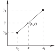
Figure \(\PageIndex{7}\)

Thus

\[\label{eq:125}\frac{y-y_{0}}{y_{1}-y_{0}}=\frac{x-x_{0}}{x_{1}-x_{0}} \]

so that, given \(x\),

\[\label{eq:126}y=y_{0}+(x-x_{0})\frac{y_{1}-y_{0}}{x_{1}-x_{0}} \]

Bilinear Interpolation

Bilinear interpolation is a two-dimensional generalization of linear interpolation. In the table below, \(f(\mathsf{D}) = f(x_{0}, y_{0}),\: f(\mathsf{A}) = f(x_{0}, y_{1}),\: f(\mathsf{F}) = f(x_{1}, y_{0})\), and \(f(\mathsf{C}) = f(x_{1}, y_{1})\) are known and \(f(x, y)\) is to be found. The bilinear interpolation technique is illustrated in the figure.

Variable
Independent	Independent	Dependent
\(x_{0}\)	\(y_{0}\)	\(f_{0}\)
\(x\)	\(y\)	\(f\)
\(x_{1}\)	\(y_{1}\)	\(f_{1}\)

Table \(\PageIndex{4}\)

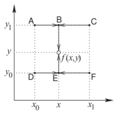
Figure \(\PageIndex{8}\)

First, find the value of the function at point \(\mathsf{B}\) from the values at Point \(\mathsf{A}\) and Point \(\mathsf{C}\). Thus, from Equation \(\eqref{eq:126}\),

\[\label{eq:127}f(\mathsf{B})=f(x,y_{1})=f(\mathsf{A})+(x-x_{0})\frac{f(\mathsf{C})-f(\mathsf{A})}{x_{1}-x_{0}} \]

Similarly

\[\label{eq:128}f(\mathsf{E})=f(x,y_{0})=f(\mathsf{D})+(x-x_{0})\frac{f(\mathsf{F})-f(\mathsf{D})}{x_{1}-x_{0}} \]

Linear interpolation between Point \(\mathsf{B}\) and Point \(\mathsf{E}\) yields

\[\label{eq:129}f(x,y)=f(\mathsf{E})+(y-y_{0})\frac{f(\mathsf{B})-f(\mathsf{E})}{y_{1}-y_{0}} \]

Combining these, the function obtained from bilinear interpolation is

\[\begin{align}f(x,y)&=\frac{f(x_{0},y_{0})}{(x_{1}-x_{0})(y_{1}-y_{0})}(x_{1}-x)(y_{1}-y)+\frac{f(x_{1},y_{0})}{(x_{1}-x_{0})(y_{1}-y_{0})}(x-x_{0})(y_{1}-y)\nonumber \\ \label{eq:130}&\quad +\frac{f(x_{0},y_{1})}{(x_{1}-x_{0})(y_{1}-y_{0})}(x_{1}-x)(y-y_{0})+\frac{f(x_{1},y_{1})}{(x_{1}-x_{0})(y_{1}-y_{0})}(x-x_{0})(y-y_{0})\end{align} \]

When interpolating from a table, choosing the points closest to the final point will yield greatest accuracy.

1.A.13 Circles on the Complex Plane

A common situation that occurs when working with complex numbers involves equating the magnitude of a complex number being equal to a real number. As will be shown, this defines a circle in the complex plane. Consider the relation

\[\label{eq:131}|S-c|=r \]

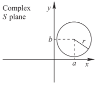
Figure \(\PageIndex{9}\): A circle in the \(S\) plane defined by the relation \(|S − c| = r\), where \(c = a + \jmath b\) and \(S = x +\jmath y\).

where \(S = x +\jmath y\) and \(c = a +\jmath b\) are complex numbers and \(r\) is a real number. Substituting for \(S\) and \(c\) in Equation \(\eqref{eq:131}\) yields

\[\begin{align}\label{eq:132} |(x − a) +\jmath (y − b)| &= r \\ \label{eq:133}\text{that is,}\quad [(x − a) +\jmath (y − b)] [(x − a) − \jmath (y − b)] &= r^{2} \\ \label{eq:134} (x − a)^{2} + (y − b)^{2} &= r^{2}\end{align} \]

The above is a general equation for a circle in the \(x-y\) plane with center \((a, b)\) and radius \(r\) (see Figure \(\PageIndex{9}\)).

1.A.14 Bilinear Transform

The bilinear transformation maps a circle in the complex plane onto another circle in the complex plane [19]. The bilinear transformation of a complex variable \(z\) is

\[\label{eq:135}w=\frac{Az+B}{Cz+1} \]

where \(A,\: B\), and \(C\) are real numbers. In RF and microwave usage, \(z\) and \(w\) could be reflection coefficients or impedances. Rearranging Equation \(\eqref{eq:133}\) results in

\[\label{eq:136}w=\frac{A}{C}+\frac{B-\frac{A}{C}}{Cz+1} \]

which can be rearranged as

\[\label{eq:137}\frac{w-\frac{A}{C}}{B-\frac{A}{C}}=\frac{1}{Cz+1} \]

The complexity of the derivation is reduced by introducing the intermediate variables \(W\) and \(Z\) defined as

\[\label{eq:138}W=\frac{w-\frac{A}{C}}{B-\frac{A}{C}} \]

and

\[\label{eq:139}Z=Cz+1 \]

and noting that, from Equation \(\eqref{eq:137}\),

\[\label{eq:140}W=1/Z \]

If, in Equation \(\eqref{eq:139}\), the locus of \(z\) describes a circle, then the locus of \(Z\) will also be a circle since \(C\) is a constant. If the center of the circle in \(Z\) space is \(C_{Z}\) and the distance from any point on the circle to the center is the radius \(R_{Z}\), then

\[\label{eq:141}|Z-C_{Z}|=R_{Z} \]

Considering Equation \(\eqref{eq:139}\), then in \(z\) space, the center of the circle is

\[\label{eq:142}C_{z}=\frac{C_{Z}}{C}-\frac{1}{C} \]

and its radius is

\[\label{eq:143}R_{z}=R_{Z}/C \]

Removing the magnitude signs in Equation \(\eqref{eq:141}\) leads to

\[\label{eq:144}(Z − C_{Z}) (Z − C_{Z})^{\ast} = (Z − C_{Z}) (Z^{\ast} − C^{\ast} Z) = R_{Z}^{2} \]

or

\[\label{eq:145}ZZ^{\ast} − C_{Z}Z^{\ast} − C_{Z}^{\ast}Z + (|CZ|^{2} − R_{Z}^{2})=0 \]

which is the general equation for a circle in the complex plane.

Now, the circle in the \(Z\) plane will be related to what happens in the \(W\) plane. Substituting Equation \(\eqref{eq:140}\) into Equation \(\eqref{eq:145}\) results in

\[\label{eq:146}\frac{1}{WW^{\ast}}-C_{Z}\frac{1}{W^{\ast}}-C_{Z}^{\ast}\frac{1}{W} + (|CZ|^{2} − R_{Z}^{2})=0 \]

and rearranging,

\[\label{eq:147}WW^{\ast}-\frac{C_{Z}}{(|C_{Z}|^{2}-R_{Z}^{2})}W-\frac{C_{Z}^{\ast}}{(|C_{Z}|^{2}-R_{Z}^{2})}W^{\ast}+\frac{1}{(|C_{Z}|^{2}-R_{Z}^{2})}=0 \]

This is in the same form as Equation \(\eqref{eq:145}\), so Equation \(\eqref{eq:147}\) describes a circle in \(W\) space with center

\[\label{eq:148}C_{W}=\frac{C_{Z}^{\ast}}{(|C_{Z}|^{2}-R_{Z}^{2})} \]

and radius

\[\label{eq:149}R_{W}=\left|\frac{R_{Z}}{|C_{Z}|^{2}-R_{Z}^{2}}\right| \]

Now the locus of \(w\) will also be a circle. From Equation \(\eqref{eq:138}\),

\[\label{eq:150}w=W\left(B-\frac{A}{C}\right)+\frac{A}{C} \]

so that \(W\) is scaled and a constant added. The center of the circle in \(w\) space is

\[\label{eq:151}C_{w}=C_{W}\left(B-\frac{A}{C}\right)+\frac{A}{C}=\frac{C_{Z}^{\ast}(B-A/C)}{(|C_{Z}|^{2}-R_{Z}^{2})}+\frac{A}{C} \]

and the radius is

\[\label{eq:152}R_{w}=R_{W}\left|B-\frac{A}{C}\right|=\left|\frac{(B-A/C)}{|C_{Z}|^{2}-R_{Z}^{2}}\right| \]

Substituting Equations \(\eqref{eq:142}\) and \(\eqref{eq:143}\) in the above relates the centers and radii in the \(w\) and \(z\) spaces:

\[\begin{align}\label{eq:153}C_{w}&=\frac{(CC_{z}+1)^{\ast}(B-A/C)}{(|CC_{z}+1|^{2}-|CR_{z}|^{2})}+\frac{A}{C} \\ \label{eq:154}R_{w}&=\left|\frac{(B-A/C)CR_{z}}{|CC_{z}+1|^{2}-|CR_{z}|^{2}}\right|=\left|\frac{(BC-A)R_{z}}{|CC_{z}+1|^{2}-|CR_{z}|^{2}}\right|\end{align} \]

Thus the bilinear transform, Equation \(\eqref{eq:135}\), maps all points on a circle in the \(z\) plane to points on a circle in the \(w\) plane.

1.A.15 Quadratic and Cubic Equations

Quadratic Equation

The general form of the quadratic equation in \(x\) is (\(a,\: b,\) and \(c\) can be complex)

\[\label{eq:155}ax^{2}+bx+c=0 \]

where \(a\neq 0\). There are two solutions, called roots, given by the quadratic formula, [20]

\[\label{eq:156}x=\frac{-b\pm\sqrt{b^{2}-4ac}}{2a} \]

and \(\pm\) indicates two possible roots,

\[\label{eq:157}x_{+}=\frac{-b+\sqrt{b^{2}-4ac}}{2a}\quad\text{and}\quad x_{-}=\frac{-b-\sqrt{b^{2}-4ac}}{2a} \]

Even if \(a,\: b\), and \(c\) are real, the roots may be complex and they could be degenerate, that is, the same. The factors of the quadratic equation come from the roots, that is,

\[\label{eq:158}ax^{2}+bx+c=a(x-x_{+})(x-x_{-}) \]

Cubic Equation

The general form of the cubic equation in \(x\) is (\(a,\: b,\: c\) and \(d\) can be complex)

\[\label{eq:159}ax^{3}+bx^{2}+cx+d=0 \]

where \(a\neq 0\). There are three solutions, called roots, given by the cubic formula, [20]

\[\label{eq:160}x_{k}=\frac{1}{3a}\left(b+u_{k}+\frac{\Delta_{0}}{u_{k}C}\right),\quad k\in\{1, 2, 3\} \]

where the \(u_{k}\)s are the cube roots of one: \(u_{1} = 1,\: u_{2} = \frac{1}{2}\left(-1+\jmath\sqrt{3}\right),\: u_{3} =\frac{1}{2}\left(−1 −\jmath\sqrt{3}\right),\) and

\[\label{eq:161}C=\left[\frac{1}{2}\left(\Delta_{1}+\sqrt{\Delta_{1}^{2}-4\Delta_{0}^{3}}\right)\right]^{1/3} \]

with \(\Delta_{0} = b^{2} − 3ac\) and \(\Delta_{1} = 2b^{3} − 9abc + 27a^{2}d\). In Equation \(\eqref{eq:161}\) any choice of the square or cube roots can be made as the effect is simply to exchange \(x_{1},\: x_{2}\) and \(x_{3}\). Note that \(ax^{3} + bx^{2} + cx + d = (x − x_{1})(x − x_{2})(x − x_{3})\).

1.A.16 Kron's Method: Network Condensation

Kron’s method [21, 22, 23] is also called network condensation and is used in developing simpler equivalent networks of large linear circuits with algebraic \(y\) parameters, that is, for resistive networks, or for general linear circuits in frequency-domain analysis where the \(y\) parameters are complex numbers. Network condensation is a numerical approach particular to circuits. It is of use in reduced-order modeling of linear circuits and in filter design.

The indefinite nodal admittance formulation of a network with four external terminals (see Figure \(\PageIndex{10}\)) is

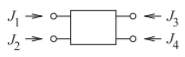
Figure \(\PageIndex{10}\): A four-terminal network.

\[\label{eq:162}\left[\begin{array}{ccccc}{y_{11}}&{y_{12}}&{\cdots}&{y_{1,k}}&{y_{1,k+1}}\\{y_{21}}&{y_{22}}&{\cdots}&{y_{2,k}}&{y_{2,k+1}}\\{\vdots}&{\vdots}&{\ddots}&{\vdots}&{\vdots}\\{y_{k1}}&{y_{k2}}&{\cdots}&{y_{k,k}}&{y_{k,k+1}}\\{y_{k+1,1}}&{y_{k+1,2}}&{\cdots}&{y_{k+1,k}}&{y_{k+1,k+1}}\end{array}\right]\left[\begin{array}{c}{v_{1}}\\{v_{2}}\\{v_{3}}\\{v_{4}}\\{v_{5}}\\{\vdots}\\{v_{k}}\\{v_{k+1}}\end{array}\right]=\left[\begin{array}{c}{J_{1}}\\{J_{2}}\\{J_{3}}\\{J_{4}}\\{0}\\{\vdots}\\{0}\\{0}\end{array}\right] \]

as there are no external current sources at the internal terminals \(5,\: 6,\:\cdots\: , k+1\). Since the \((k+1)\)th current source is zero, the \((k + 1)\)th row and column of \(\mathbf{Y}\) can be eliminated, yielding

\[\label{eq:163}\left[\begin{array}{cccc}{y_{11}'}&{y_{12}'}&{\cdots}&{y_{1,k}'}\\{y_{21}'}&{y_{22}'}&{\cdots}&{y_{2,k}'}\\{\vdots}&{\vdots}&{\ddots}&{\vdots}\\{y_{k1}'}&{y_{k2}'}&{\cdots}&{y_{k,k}'}\end{array}\right]\left[\begin{array}{c}{v_{1}'}\\{v_{2}'}\\{v_{3}'}\\{v_{4}'}\\{v_{5}'}\\{\vdots}\\{v_{k}'}\end{array}\right]=\left[\begin{array}{c}{J_{1}}\\{J_{2}}\\{J_{3}}\\{J_{4}}\\{0}\\{\vdots}\\{0}\end{array}\right] \]

where

\[\label{eq:164}y_{ij}'=y_{ij}-y_{k+1, j}\frac{y_{i,k+1}}{y_{k+1,k+1}}\quad\text{and}\quad v_{i}'=v_{i}-v_{k+1} \]

It is of no concern that the terminal voltages have been altered, as they have all had the same quantity added to them. This has the same effect as choosing another reference terminal. The reference terminal is arbitrary until it is connected to the full circuit. The process can be continued until the network equations are reduced to that of a four-terminal element, that is

\[\label{eq:165}\left[\begin{array}{cccc}{y_{11}''}&{y_{12}''}&{y_{13}''}&{y_{14}''}\\{y_{21}''}&{y_{22}''}&{y_{23}''}&{y_{24}''}\\{y_{31}''}&{y_{32}''}&{y_{33}''}&{y_{34}''}\\{y_{41}''}&{y_{42}''}&{y_{43}''}&{y_{44}''}\end{array}\right]\left[\begin{array}{c}{v_{1}''}\\{v_{2}''}\\{v_{3}''}\\{v_{4}''}\end{array}\right]=\left[\begin{array}{c}{J_{1}}\\{J_{2}}\\{J_{3}}\\{J_{4}}\end{array}\right] \]

The \(y\)-parameter matrix in Equation \(\eqref{eq:165}\) is that of the four-terminal element shown in Figure \(\PageIndex{10}\).

Footnotes

[1] Outside electrical engineering \(\imath\) (\(i\) without the dot) is used for \(\sqrt{−1}\), but this is replaced by \(\jmath\) (\(j\) without the dot) in electrical engineering to avoid confusion with the usage of \(i\) for current.