
2.5: The Lossy Terminated Line
- Page ID
- 41016

Previously Section 2.3 presented abstractions that enabled a total voltage and current view to be used with lossless transmission lines. A similar development is presented here for lossy lines. Important abstractions are presented first for the input reflection coefficient of a terminated lossy line in Section 2.5.1 and then for the input impedance of first a long lossy line in Section 2.5.2 and then for a finite length line in Section 2.5.3. Section 2.5.4 presents a simple approximation for the attenuation on a line if it is low loss. Power flow on a lossy line is considered in Section 2.5.5 and then the impact of dispersion on signal integrity considered in Section 2.5.6. The final section, Section 2.5.7, describes a technique for the design of a finite bandwidth dispersion-less line.
2.5.1 Input Reflection Coefficient of a Lossy Line
\(\Gamma_{\text{in}}\) of a lossy line can be developed by replacing \(\jmath\beta\) in Section 2.3.3 by \(\gamma\). Referring to Figure 2.3.4, at a distance \(\ell\) from the load (i.e., \(z = −\ell\)), the input reflection looking into a lossy line toward the load is
\[\begin{align}\left.\Gamma_{\text{in}}\right|_{z=-\ell}&=\frac{ V ^{-}(z = −\ell)}{ V ^{+}(z = −\ell)}=\frac{V ^{−}(z = 0)e^{−\gamma\ell}}{V ^{+}(z = 0)e^{+\gamma\ell}}=\frac{V ^{−}(z = 0)e^{−\gamma\ell}}{V ^{+}(z = 0)e^{+\gamma\ell}}\nonumber \\ \label{eq:1} &=\Gamma_{L}e^{-2\gamma\ell}=\Gamma_{L}e^{-2\alpha\ell}e^{-2\jmath\beta\ell}\end{align} \]
As the line becomes longer the magnitude of \(\Gamma_{\text{in}}\) decreases exponentially, approaching zero, because of attenuation described by the \(e^{−2\alpha\ell}\) term.
2.5.2 Input Impedance of a Long Lossy Line
Figure \(\PageIndex{1}\)(a) shows an infinitely long line with characteristic impedance \(Z_{0}\). The input impedance \(Z_{\text{in}}\) of the line is the ratio of the total voltage \(V_{1}\) to the total current \(I_{1}\) at the input of the line:
\[\label{eq:2} Z_{\text{in}}=\frac{V_{1}}{I_{1}} \]
If the line is infinitely long or sufficiently lossy there is negligible reflected wave and thus the total voltage and current are just the forward-traveling
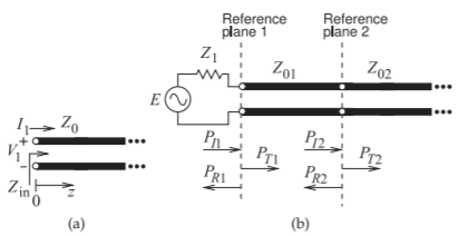
Figure \(\PageIndex{1}\): Transmission line networks: (a) an infinitely long line; and (b) with a finite-length line of characteristic impedance \(Z_{01}\) and an infinitely long transmission line of characteristic impedance \(Z_{02}\).
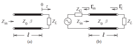
Figure \(\PageIndex{2}\): Terminated transmission line: (a) a transmission line terminated in a load impedance, \(Z_{L}\), with an input impedance of \(Z_{\text{in}}\); and (b) a transmission line with source impedance \(Z_{G}\) and load \(Z_{L}\).
voltage and current and
\[\label{eq:3}Z_{\text{in}}=\frac{V_{1}}{I_{1}}=\frac{V^{+}(0)}{I^{+}(0)}=Z_{0} \]
The infinitely long line is approximated by a very long, slightly lossy, cable. It will not matter how the line is terminated (e.g., in a resistor, open circuit, or short circuit), there will be a negligible backward-traveling wave, and the input impedance of the cable will be its characteristic impedance.
2.5.3 Input Impedance of a Lossy Line
The impedance looking into the line varies with position, as the forwardand backward-traveling waves combine to yield position-dependent total voltage and current. At a distance \(\ell\) from the load (i.e., \(z = −\ell\)), the input impedance seen looking toward the load is
\[\label{eq:4}\left. Z_{\text{in}}\right|_{z=-\ell}=\frac{V(z=-\ell)}{I(z=-\ell)}=Z_{0}\frac{1+|\Gamma|e^{(\jmath\Theta -2\gamma\ell)}}{1-|\Gamma|e^{(\jmath\Theta -2\gamma\ell)}}=Z_{0}\frac{1+\Gamma_{L}e^{-2\gamma\ell}}{1-\Gamma_{L}e^{-2\gamma\ell}} \]
Another form comes from substituting Equation (2.3.6) in Equation \(\eqref{eq:4}\):
\[\begin{align}Z_{\text{in}}&=Z_{0}\frac{(Z_{L} + Z_{0})e^{\gamma\ell} + (Z_{L} − Z_{0})e^{−\gamma\ell}}{(Z_{L} + Z_{0})e^{\gamma\ell} − (Z_{L} − Z_{0})e^{−\gamma\ell}}=Z_{0}\frac{Z_{L} \cosh(\gamma\ell) + \jmath Z_{0} \cosh(\gamma\ell)}{Z_{0} \cosh(\gamma\ell) +\jmath Z_{L} \cosh(\gamma\ell)}\nonumber \\ \label{eq:5} &=Z_{0}\frac{Z_{L} + Z_{0} \tanh\gamma\ell}{Z_{0} + Z_{L} \tanh\gamma\ell}\end{align} \]
This equation is also known as the lossy telegrapher’s equation.
Note that \(Z_{\text{in}}\) is a quasi-periodic function of \(\ell\) and approaches \(Z_{0}\) for a long lossy line (i.e. provided that there is attenuation and the line’s \(\gamma\) has a real part as then \(\tanh\gamma\ell\) goes to one).
A shorted line is used as a resonator. The first resonance is a parallel resonance at \(1\text{ GHz}\).
- Draw the lumped-element equivalent circuit of the resonator.
- What is the impedance looking into the line at resonance?
- What is the electrical length of the resonator?
- If the resonator is \(\lambda_{g}/4\) longer, what is the input impedance of the resonator now?
Solution
-

Figure \(\PageIndex{3}\)
\(LC\) is an open circuit at resonance. If the line is lossless, \(R=0\). - \(Z_{\text{in}}=\infty\) (for a lossless line).
- From Equation (2.3.18) and with \(Z_{L = 0}\), \(Z_{\text{in}} = \jmath Z_{0} \tan(\beta\ell)\). \(Z_{\text{in}} = \infty\) when \(\tan(\beta\ell) =\infty\), i.e. when \(\beta\ell = π/2 = \lambda_{g}/4 = 90^{\circ}\).

Figure \(\PageIndex{4}\) - \(Z_{\text{in}}=0\:\Omega\)
2.5.4 Attenuation on a Low-Loss Line
Recall that \(\gamma\), the propagation constant, is given by
\[\label{eq:6}\gamma=\sqrt{(R+\jmath\omega L)(G+\jmath\omega C)} \]
This can be written as
\[\label{eq:7}\gamma =\jmath\omega\sqrt{LC}\sqrt{\left(1+\frac{R}{\jmath\omega L}\right)\left(1+\frac{G}{\jmath\omega C}\right)} \]
With a low-loss line, \(R ≪ \omega L\) and \(G ≪ \omega C\), and so, using a Taylor series approximation (see Equation (1.A.88)),
\[\label{eq:8}\left(1+\frac{R}{\jmath\omega L}\right)^{1/2}\approx 1+\frac{1}{2}\frac{R}{\jmath\omega L} \]
and
\[\label{eq:9}\left(1+\frac{G}{\jmath\omega C}\right)^{1/2}\approx 1+\frac{1}{2}\frac{G}{\jmath\omega C} \]
thus
\[\label{eq:10}\gamma\approx\frac{1}{2}\left(R\sqrt{\frac{C}{L}}+G\sqrt{\frac{L}{C}}\right)+\jmath\omega\sqrt{LC} \]
Hence for low-loss lines (in \(\text{Np/m}\) if SI units are used),
\[\label{eq:11}\alpha\approx\frac{1}{2}\left(\frac{R}{Z_{0}}+GZ_{0}\right) \]
and
\[\label{eq:12}\beta\approx\omega\sqrt{LC} \]
What Equation \(\eqref{eq:11}\) indicates is that for low-loss lines the attenuation constant, \(\alpha\), consists of dielectric- and conductor-related parts; that is,
\[\label{eq:13}\alpha =\alpha_{d}+\alpha_{C} \]
\[\label{eq:14}\alpha_{d}\approx GZ_{0}/2 \]
and
\[\label{eq:15}\alpha_{c}\approx R/(2Z_{0}) \]
where \(\alpha_{d}\) is the attenuation contributed by dielectric loss and is called dielectric attenuation, and \(\alpha_{d}\) is the attenuation contributed by the conductor loss and is called ohmic or conductive attenuation.
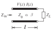
Figure \(\PageIndex{5}\): A low-loss transmission line. The propagation constant \(\gamma =\alpha+\jmath\beta\).
2.5.5 Power Flow on a Terminated Lossy Line
In this section a lossy transmission line with low loss is considered so that \(R ≪ \omega L\) and \(G ≪ \omega C\), and the characteristic impedance is \(Z_{0} \approx\sqrt{L/C}\). Figure \(\PageIndex{5}\) is a lossy transmission line and the total voltage and current at any point on the line are given by
\[\label{eq:16}V(z)=V_{0}^{+}\left[e^{-\gamma z}+\Gamma e^{\gamma z}\right]\quad\text{and}\quad I(z)=\frac{V_{0}^{+}}{Z_{0}}\left[e^{-\gamma z}-\Gamma e^{\gamma z}\right] \]
Section 2.5.3 derived the lossy telegrapher’s equation:
\[\label{eq:17}Z_{\text{in}}=Z_{0}\frac{Z_{L} + Z_{0} \tanh\gamma\ell}{Z_{0} + Z_{L} \tanh\gamma\ell} \]
For a lossy transmission line not all of the power applied at the input will be delivered to the load as power will be lost on the line due to attenuation. The power delivered to the load (which is at position \(z = 0\)) is
\[\label{eq:18}P_{L}=\frac{1}{2}\mathcal{R}\{V(0)I^{\ast}(0)\}=\frac{|V_{0}^{+}|^{2}}{2Z_{0}}(1-|\Gamma_{L}|^{2}) \]
where \(\Gamma_{L}\) is the reflection coefficient of the load. Similarly the power at the input of the line (at position \(z = −\ell\)) is
\[\label{eq:19}P_{\text{in}}=\frac{1}{2}\Re\{V(-\ell)I^{\ast}(-\ell)\}=\frac{|V_{0}^{+}|^{2}}{2Z_{0}}[1-|\Gamma_{L}|^{2}e^{-4\alpha\ell}]e^{2\alpha\ell} \]
and the power lost in the line is
\[\label{eq:20}P_{\text{loss}}=P_{\text{in}}-P_{L}=\frac{|V_{0}^{+}|^{2}}{2Z_{0}}[(e^{2\alpha\ell}-1)+|\Gamma_{L}|^{2}(1-2^{-2\alpha\ell})] \]
Energy is stored on a transmission line and this must be considered in deriving the \(Q\) of a transmission line resonator. Consider the \(\lambda/4\)- long shorted transmission line examined in Examples 2.3.1 and 2.4.2. This line has a characteristic impedance of \(12.28\:\Omega\), it is resonant at \(1850\text{ MHz}\), and a \(10\text{ k}\Omega\) resistor, \(R\), is at the input as shown in the left figure.
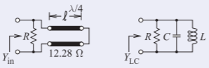
Figure \(\PageIndex{6}\)
Solution
At resonance
\[\begin{align} \label{eq:21}Q&=2\pi\frac{\text{Peak energy stored}}{\text{Energy dissipated per cycle}}=\omega_{r}\frac{\text{Peak energy stored}}{\text{Power loss in the resistor}} \\ \label{eq:22}Q&=1/(\text{Fractional bandwidth})\end{align} \]
where \(\omega_{r}\) is the radian frequency at resonance. So there are two fundamental ways that the \(Q\) can be determined: determining the peak energy stored and the power loss, and finding the fractional bandwidth. However, using the fractional bandwidth is only an approximate method, as \(Q\) is a measure of energy stored and energy dissipated.
For an \(RLC\) lumped-element resonator
\[\label{eq:23}Q=\left\{\begin{array}{ll}{\frac{1}{R}\sqrt{\frac{L}{C}}=\frac{\omega_{r}L}{R}}&{\text{for a series }RLC\text{ circuit}}\\{R\sqrt{\frac{C}{L}}=\frac{\omega_{r}C}{G}}&{\text{for a shunt }RLC\text{ circuit}}\end{array}\right. \]
The narrowband lumped-element equivalent circuit of the resonator developed in Example 2.3.1, with \(C = 5.503\text{ pF}\) and \(L = 1.345\text{ pH}\) can be used. Thus
\[Q=R\sqrt{\frac{C}{L}}=10\cdot 10^{3}\sqrt{\frac{5.503\cdot 10^{-12}}{1.345\cdot 10^{-9}}}=640\nonumber \]
It is important to note that the input impedance of the transmission line at the resonant frequency cannot be used to find the \(Q\) of the transmission line resonator, as it does not convey any information about the energy stored. However, the narrowband model of the resonator at resonance does capture the energy storage information and so can be used to calculate the \(Q\) of the resonator, as was done here.
2.5.6 Lossy Transmission Line Dispersion
On a lossy line, phase velocity, group velocity, and attenuation constant are frequency dependent and so a lossy line is, in general, dispersive. That is, different frequency components of a signal travel at different speeds, and the phase velocity, \(v_{p}\), and group velocity, \(v_{g}\), are functions of frequency. As a result, the signal will spread out in time and, if the line is long enough, it will be difficult to extract the original information.
In the previous section it was seen, in Equation \(\eqref{eq:12}\), that for a TEM line \(\omega /\beta = v_{p} = v_{g}\) is approximately frequency independent for a low-loss line. This is true for most two-conductor lines (lines that support TEM modes), but not for all transmission line structures that guide EM waves (a rectangular waveguide is an example of where \(v_{g}\) and \(v_{p}\) differ significantly). Also, the conductive component of the attenuation constant, \(\alpha_{c}\) in Equation \(\eqref{eq:15}\), is approximately frequency independent. However, the dielectric component, \(\alpha_{d}\) in Equation \(\eqref{eq:14}\), is frequency dependent even for a low-loss line. This is because \(G\) is mostly due to energy loss when a material lattice or molecular components are distorted by the \(E\) field. So there is more loss and \(G\) increases linearly as the frequency increases. (Conductivity of the dielectric also affects \(G\), but this is usually a much smaller effect except for a silicon substrate.) If the transmission line has moderate loss, all of the propagation parameters will be frequency dependent and the line is dispersive.
2.5.7 Design of a Dispersionless Lossy Line
Over a moderate bandwidth a lossy line can be designed to be dispersionless (i.e. \(v_{g}\approx v_{p}\approx\) constant). The parameters that are important in describing signal propagation on a transmission line are the propagation constant, \(\gamma\), and the characteristic impedance, \(Z_{0}\). When considering dispersion it is more appropriate to examine \(\alpha\) and \(v_{p}\approx\omega/\beta\) (for a low loss line), as these parameters are generally frequency dependent for a lossy line. For a line to be dispersionless \(\alpha\), \(\omega/\beta\), and \(Z_{0}\) should be independent of frequency.
For any low-loss line the propagation constant is
\[\label{eq:24}\gamma=\sqrt{(R+\jmath\omega L)(G+\jmath\omega C)}=\jmath\omega\sqrt{LC}\left[\left(1+\frac{R}{\jmath\omega L}\right)\left(1+\frac{G}{\jmath\omega C}\right)\right]^{1/2} \]
If the line is designed so that
\[\label{eq:25}R/L=G/C \]
then
\[\label{eq:26}\gamma=\alpha+\jmath\beta=\jmath\omega\sqrt{LC}\left(1+\frac{R}{\jmath\omega L}\right)=R\sqrt{\frac{C}{L}}+\jmath\omega\sqrt{LC} \]
From this
\[\label{eq:27}\alpha=R\sqrt{\frac{C}{L}},\:\beta=\omega\sqrt{LC}\text{ and }v_{p}=\omega/\beta=1/\sqrt{LC} \]
The analysis is completed by considering the characteristic impedance
\[\label{eq:28}Z_{0}=\sqrt{\frac{R+\jmath\omega L}{G+\jmath\omega C}}=\sqrt{\frac{L}{C}}\sqrt{\frac{R/L+\jmath\omega}{G/C+\jmath\omega}} \]
and, referring to Equation \(\eqref{eq:25}\), note that the last square root term is \(1\), so
\[\label{eq:29}Z_{0}=\sqrt{L/C} \]
which is frequency independent. The important characteristics describing signal propagation are now frequency independent and the line is dispersionless. In practice a lossy dispersionless line can only be approximated over a small bandwidth since \(G\) is linearly dependent on frequency because of the frequency dependence of dielectric relaxation loss.
2.5.8 Summary
An earlier section developed the input reflection coefficient and input impedance of a lossless line. This section did the same thing but for a lossy line. Short-hand derivations were presented for the attenuation of a low loss line in terms of the per-unit-length resistance and characteristic impedance of the line. Dispersion on a line was discussed and a design technique presented for the design of a dispersionless line. This design is valid over a narrow or moderate bandwidth and this bandwidth limitation applies to all transmission line-based designs.