2.8: Two-Conductor Transmission Lines

Last updated
Save as PDF

Page ID: 41022

\( \newcommand{\vecs}[1]{\overset { \scriptstyle \rightharpoonup} {\mathbf{#1}} } \) \( \newcommand{\vecd}[1]{\overset{-\!-\!\rightharpoonup}{\vphantom{a}\smash {#1}}} \)\(\newcommand{\id}{\mathrm{id}}\) \( \newcommand{\Span}{\mathrm{span}}\) \( \newcommand{\kernel}{\mathrm{null}\,}\) \( \newcommand{\range}{\mathrm{range}\,}\) \( \newcommand{\RealPart}{\mathrm{Re}}\) \( \newcommand{\ImaginaryPart}{\mathrm{Im}}\) \( \newcommand{\Argument}{\mathrm{Arg}}\) \( \newcommand{\norm}[1]{\| #1 \|}\) \( \newcommand{\inner}[2]{\langle #1, #2 \rangle}\) \( \newcommand{\Span}{\mathrm{span}}\) \(\newcommand{\id}{\mathrm{id}}\) \( \newcommand{\Span}{\mathrm{span}}\) \( \newcommand{\kernel}{\mathrm{null}\,}\) \( \newcommand{\range}{\mathrm{range}\,}\) \( \newcommand{\RealPart}{\mathrm{Re}}\) \( \newcommand{\ImaginaryPart}{\mathrm{Im}}\) \( \newcommand{\Argument}{\mathrm{Arg}}\) \( \newcommand{\norm}[1]{\| #1 \|}\) \( \newcommand{\inner}[2]{\langle #1, #2 \rangle}\) \( \newcommand{\Span}{\mathrm{span}}\)\(\newcommand{\AA}{\unicode[.8,0]{x212B}}\)

Nearly every two-conductor transmission line supports EM fields at frequencies down to DC. As a result, such lines can usually be characterized at DC and the properties of the lines will be essentially the same at RF frequencies. In the following, the characteristic impedances of the most common types of two-conductor lines are presented. For all of these lines the phase constant is the same as it would be in the medium without conductors (i.e., \(\beta =\omega\sqrt{\mu\varepsilon}\)). The characteristic impedances are modifications of the freespace wave impedance \(\eta_{0} =\sqrt{\mu_{0}/\varepsilon_{0}} = 120\pi\:\Omega = 376.73\:\Omega\). The properties of many other transmission lines are given in [8].

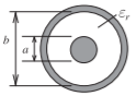
Figure \(\PageIndex{1}\): Coaxial line

\[\label{eq:1}Z_{0}=\frac{\eta_{0}}{2\pi}\sqrt{\frac{\mu_{r}}{\varepsilon_{r}}}\ln\left(\frac{b}{a}\right)=60\sqrt{\frac{\mu_{r}}{\varepsilon_{r}}}\ln\left(\frac{b}{a}\right) \]

Exact. See derivation in Section 2.9.

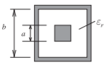
Figure \(\PageIndex{2}\): Square coaxial line

\[\label{eq:2}Z_{0}\approx\eta_{0}\sqrt{\frac{\mu_{r}}{\varepsilon_{r}}}\left[4\left(\frac{2a}{b-a}+0.558\right)\right]^{-1} \]

Typical accuracy: \(<1\%\) for \(b/a\leq 4\). Reference [9].

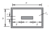
Figure \(\PageIndex{3}\): Rectangular coaxial line

\[\label{eq:3}Z_{0}=\frac{\eta_{0}}{4}\sqrt{\frac{\mu_{r}}{\varepsilon_{r}}}\left(\frac{\omega}{b-t}+\frac{1}{\pi}\left\{\frac{b}{b-t}\ln\left(\frac{2b-t}{t}\right)+\ln\left[\frac{t(2b-t)}{(b-t)^{2}}\right]\right\}\frac{\ln[1+\coth(\pi g/b)]}{\ln 2}\right)^{-1} \]

Typical accuracy: \(1\%\). References [10, 11, 12].

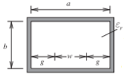
Figure \(\PageIndex{4}\): Rectangular coaxial line, thin strip \(t\to 0\)

\[\label{eq:4}Z_{0}=\frac{\eta_{0}}{4}\sqrt{\frac{\mu_{r}}{\varepsilon_{r}}}\left\{\frac{\omega}{b}+\frac{2}{\pi}\ln\left[1+\coth\left(\frac{\pi g}{b}\right)\right]\right\}^{-1} \]

Typical accuracy: \(1\%\). Reference [10].

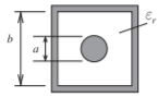
Figure \(\PageIndex{5}\): Square coax with circular inner conductor

\[\label{eq:5}Z_{0}=\frac{\eta_{0}}{2\pi}\sqrt{\frac{\mu_{r}}{\varepsilon_{r}}}\ln\left(\frac{1.0787b}{a}\right) \]

Typical accuracy: \(1.5\%\). References [8, 13, 14, 15].

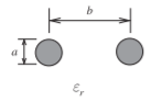
Figure \(\PageIndex{6}\): Parallel wires

\[\label{eq:6}Z_{0}=\frac{\eta_{0}}{\pi}\sqrt{\frac{\mu_{r}}{\varepsilon_{r}}}\text{arccosh}\left(\frac{b}{a}\right) \]

Typical accuracy: \(1\%\). References [16, 17].

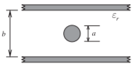
Figure \(\PageIndex{7}\): Slab line

\[\label{eq:7}Z_{0}=15\sqrt{\frac{\mu_{r}}{\varepsilon_{r}}}\ln\left[1+1.314g+\sqrt{(1.314g)^{2}+2g}\right]\quad\text{where }g=(b/a)^{4}-1 \]

Typical accuracy: \(0.5\%\). Reference [18].

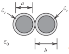
Figure \(\PageIndex{8}\): Twisted pair with \(T\) twists per unit length

\[\begin{align}\label{eq:8}Z_{0}&=\frac{\eta_{0}}{\pi}\sqrt{\frac{\mu_{r}}{\varepsilon_{e}}}\text{arccosh}\left(\frac{b}{a}\right) \\ \varepsilon_{e}&=1+q(\varepsilon_{r}-1),\: q=0.25+0.0004\Theta^{2} \\ T&=\frac{\tan\Theta}{\pi D}\text{ so }\Theta -\arctan(T\pi D)\nonumber\end{align} \nonumber \]

Typical accuracy: \(1\%\). Reference [19].

Characteristics of two-conductor transmission lines.