
4.3: High-Frequency Properties of Microstrip Lines
- Page ID
- 41038

Here the high-frequency properties of microstrip lines are discussed and formulas incorporating frequency dependence are presented for effective permittivity, characteristic impedance, and attenuation loss. The effective permittivity at DC (as calculated in the previous chapter) is denoted \(\varepsilon_{e}(0)\) and the characteristic impedance at DC is \(Z_{0}(0)\). These are also called the quasi-static effective permittivity and quasi-static characteristic impedance. Detailed analysis [12] yields the following formula for the frequency-dependent effective permittivity of a microstrip line:
\[\label{eq:1}\varepsilon_{e}(f)=\varepsilon_{r}-\frac{\varepsilon_{r}-\varepsilon_{e}(0)}{1+(f/f_{a})^{m}} \]
where
\[\begin{align} \label{eq:2}f_{a}&=\frac{f_{b}}{0.75 + (0.75 − 0.332 \varepsilon_{r}^{−1.73}) (w/h)} \\ \label{eq:3} f_{b}&=\frac{47.746 \times 10^{6}}{h\sqrt{\varepsilon_{r}-\varepsilon_{e}(0)}}\tan^{-1}\left\{\varepsilon_{r}\sqrt{\frac{\varepsilon_{e}(0)-1}{\varepsilon_{r}-\varepsilon_{e}(0)}}\right\} \\ \label{eq:4}m&=\left\{\begin{array}{ll}{m_{0}m_{c}}&{m_{0}m_{c}\leq 2.32}\\{2.32}&{m_{0}m_{c}>2.32}\end{array}\right. \\ \label{eq:5}m_{0}&=1+\frac{1}{1+\sqrt{w/h}}+0.32\left(1+\sqrt{w/h}\right)^{-3} \\ \label{eq:6}m_{c}&=\left\{\begin{array}{ll}{1+\frac{1.4}{1+w/h}\{0.15-0.235e^{-0.45f/f_{a}}\}}&{\text{for }w/h\leq 0.7}\\{1}&{\text{for }w/h>0.7}\end{array}\right. \end{align} \]
SI units are used in these equations. The accuracy of the equations is better than \(0.6\%\) for \(0.1\leq w/h\leq 10\), \(1\leq\varepsilon_{r}\leq 128\), and for any value of \(h/\lambda\) provided that \(h < \lambda /10\).
The free-space wavelength is \(\lambda_{0}\), the wavelength in the medium is \(\lambda\), and the guide wavelength (the wavelength on the line) is \(\lambda_{g}\).
The frequency-dependent characteristic impedance is, with reference to Equations (3.5.13) and (3.5.12),
\[\label{eq:7} Z_{0}(f)=\frac{Z_{01}}{\sqrt{\varepsilon_{e}(f)}}=Z_{0}(0)\frac{\sqrt{\varepsilon_{e}(0)}}{\sqrt{\varepsilon_{e}(f)}} \]
4.3.1 Frequency-Dependent Loss
The effect of loss on signal transmission is captured by the attenuation constant, \(\alpha\). There are two primary sources of loss: that resulting from the dielectric, captured by the dielectric attenuation constant, \(\alpha_{d}\), and that from the conductor loss, captured by the conductor attenuation constant, \(\alpha_{c}\). Thus
\[\label{eq:8}\alpha|_{\text{dB}}=\alpha_{d}|_{\text{dB}}+\alpha_{c}|_{\text{dB}} \]
When dielectric loss is significant (e.g., the substrate is silicon which has appreciable conductivity), the previous formula for \(\alpha_{d}\) (Equation (3.5.26)) provides a good estimate for the attenuation when \(\varepsilon_{e}\) is replaced by the frequency-dependent effective relative permittivity, \(\varepsilon_{e}(f)\).
Frequency-dependent conductor loss, described by the conductor attenuation \(\alpha_{c}\), results from the concentration of current as frequency increases:
\[\label{eq:9}\alpha_{c}(f)=\frac{R(f)}{2Z_{0}} \]
where \(R(f)\) is the frequency-dependent line resistance described in Section 4.2.5.
A third source of loss is radiation loss, leading to an attenuation factor, \(\alpha_{r}\). At the frequencies at which a transmission line is generally used, it is usually smaller than dielectric and conductor losses. So, in full,
\[\label{eq:10}\alpha(f)=\alpha_{d}(f)\cdot\alpha_{c}(f)\cdot\alpha_{r}(f) \]
and in decibels
\[\label{eq:11}\alpha(f)|_{\text{dB}}=\alpha_{d}(f)|_{\text{dB}}+\alpha_{c}(f)|_{\text{dB}}+\alpha_{r}(f)|_{\text{dB}} \]
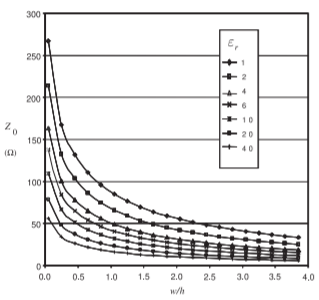
Figure \(\PageIndex{1}\): Dependence of \(Z_{0}\) of a microstrip line at \(1\text{ GHz}\) for various permittivities and aspect \((w/h)\) ratios.
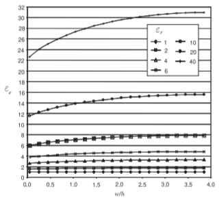
Figure \(\PageIndex{2}\): Dependence of effective relative permittivity, \(\varepsilon_{e}\), of a microstrip line at \(1\text{ GHz}\) for various permittivities and aspect ratios \((w/h)\).
4.3.2 Field Simulations
In this section, results are presented for EM simulations of microstrip lines with a variety of parameters. These simulations were performed using the Sonnet EM simulator. Figure \(\PageIndex{1}\) presents calculations of \(Z_{0}\) for various aspect ratios \((w/h)\) and substrate permittivities \((\varepsilon_{r})\) when there is no loss. The key information here is that narrow strips and low-permittivity substrates have high \(Z_{0}\). Conversely, wide strips and high-permittivity substrates have low \(Z_{0}\). The dependence of permittivity on aspect ratio is shown in Figure \(\PageIndex{2}\), where it can be seen that the effective permittivity, \(\varepsilon_{e}\), increases for wide strips. This is because more of the EM field is in the substrate.
When loss is incorporated, \(\varepsilon_{e}\) becomes complex and the imaginary components indicate loss mostly due to conductor loss. Figure \(\PageIndex{3}\) presents the frequency dependence of three microstrip lines with different substrates and aspect ratios. These simulations took into account finite loss in the conductors and in the dielectric. In Figure \(\PageIndex{3}\)(a) it can be seen that the effective permittivity, \(\varepsilon_{e}\), increases with frequency as the fields become confined more to the substrate. Also, the real part of the characteristic impedance is plotted with respect to frequency. Up to \(20\text{ GHz}\) a drop-off in \(Z_{0}\) is observed as frequency increases. This is due to both reduction of internal strip and ground inductances as charges move to the skin of the conductor and also to greater confinement of the EM fields in the dielectric as frequency increases. It is not long before the characteristic impedance increases. This effect is not due to the skin effect and current bunching that were previously described. Rather it is due to other EM effects that are only captured in EM simulation. It is a result of spatial variations being developed in the fields (related to the fact that not all parts of the fields are in instantaneous contact).
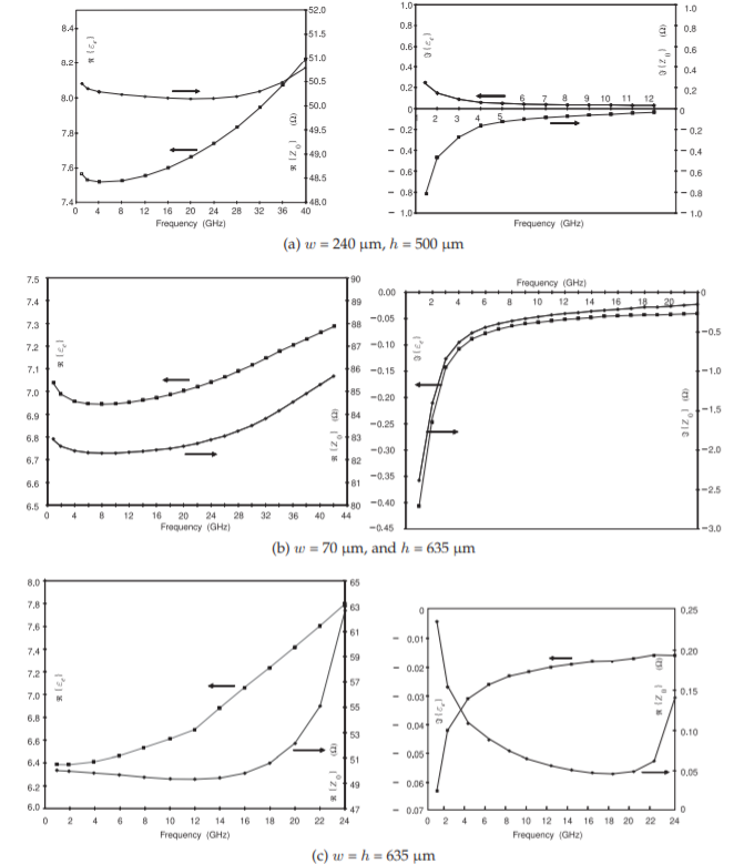
Figure \(\PageIndex{3}\): Frequency dependence of the real and imaginary parts of \(\varepsilon_{e}\) and \(Z_{0}\) of a gold microstrip line on alumina with \(\varepsilon_{r}\)(DC).
4.3.3 Summary
Today’s microwave designer is indeed fortunate that in the 1980s considerable effort was put into developing frequency-dependent formulas for effective permittivity and characteristic impedance, Equations \(\eqref{eq:1}\) and \(\eqref{eq:7}\), and these can still be used. One effect that is not captured by these formulas is the increased transverse curl of the EM fields with increasing frequency and this tends to increase the characteristic impedance, e.g. see Section 4.3.2. But the frequency-dependence of effective relative permittivity is captured. To incorporate the geometric impact on frequency-dependent characteristic impedance it is necessary to optimize a design using EM field simulation following an initial design using the frequency-dependent formulas.