5.4: Low Frequency Capacitance Model of Coupled Lines

The low-frequency model of a pair of lossless coupled lines comprises only capacitances. A pair of coupled lines, as shown in Figure \(\PageIndex{1}\)(a), has four terminals. At very low frequencies \(V_{1}\) and \(V_{3}\) are identical as are voltages \(V_{2}\) and \(V_{4}\). So the low-frequency model of the pair of coupled lines has just two terminals in addition to ground, as shown in Figure \(\PageIndex{1}\)(b).

The capacitances in Figure \(\PageIndex{1}\)(b) are the shunt capacitance \(C_{1}\) and \(C_{2}\) and the mutual capacitance \(C_{g}\). In the even mode, the voltages at terminals \(\mathsf{1}\) and \(\mathsf{2}\) are the same so that \(C_{g}\) vanishes and the low-frequency capacitance model of the pair of coupled lines in the even mode comprises just the self-capacitances \(C_{1}\) and \(C_{2}\) (see Figure \(\PageIndex{1}\)(c)). In the odd mode, the voltage at terminal \(\mathsf{2}\) is the negative of the voltage at terminal \(\mathsf{1}\). The result is that there is a virtual ground between the terminals. Now a better circuit model is that shown in Figure \(\PageIndex{1}\)(d). This is where the restriction that the lines are of equal width is used. This assumption places the virtual ground between equal-value capacitances. The symmetrical case is the one of most interest. If asymmetrical coupled lines are to be analyzed, the analysis departs at this point and EM simulation is required.

To proceed, the capacitance model must be put in the form of per unit length capacitances and put in terms of the elements of a capacitance matrix.

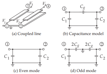
Figure \(\PageIndex{1}\): Very low frequency models of a pair of coupled lines.

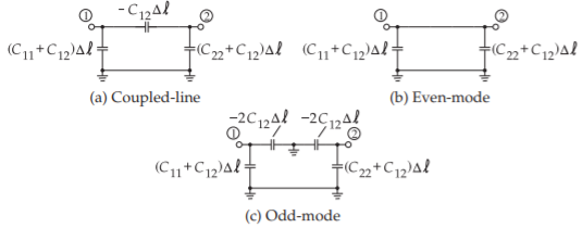
Figure \(\PageIndex{2}\): Low frequency capacitance models of a pair of coupled lines of length \(\Delta\ell\).

The indefinite nodal admittance matrix of the low-frequency coupled-line model of Figure \(\PageIndex{1}\)(b) is

\[\label{eq:1}\mathbf{Y}=\jmath\omega\left[\begin{array}{cc}{C_{1}+C_{g}}&{-C_{g}}\\{-C_{g}}&{C_{2}-C_{g}}\end{array}\right]=\jmath\omega\mathbf{C}\Delta\ell \]

where \(\Delta\ell\) is the length of the coupled lines, and \(\mathbf{C}\) is the per unit length capacitance matrix (see Equation (5.3.5)). Thus the low-frequency capacitance model of a pair of coupled lines of length \(\Delta\ell\) and equal width is as shown in Figure \(\PageIndex{2}\)(a). It is found in analysis that \(C_{12}\) is negative.

For symmetrical coupled lines (the strips having the same width) the per unit length even- and odd-mode capacitances, as defined in the definition of odd and even modes in Section 5.2, are

\[\label{eq:2}C_{e}=C_{11}+C_{12}\quad\text{and}\quad C_{o}=C_{11}-C_{12} \]

That is,

\[\label{eq:3}\mathbf{C}=\left[\begin{array}{cc}{C_{11}}&{C_{12}}\\{C_{12}}&{C_{22}}\end{array}\right]=\left[\begin{array}{cc}{\frac{1}{2}(C_{e}+C_{o})}&{\frac{1}{2}(C_{e}-C_{o})}\\{\frac{1}{2}(C_{e}-C_{o})}&{\frac{1}{2}(C_{e}+C_{o})}\end{array}\right] \]

5.4.1 Capacitance Matrix Extraction

This section describes a general procedure for the extraction of the capacitance matrix of a number of coupled conductors [1]. Either measurements or measurement-like simulations can be used. This is done by evaluating one capacitance at a time for different connections of interconnects to each other.

Without loss of generality, consider the three-line structure shown in Figure \(\PageIndex{3}\), where there are four conductors, including ground. A \(3\times 3\) capacitance matrix is extracted from the capacitances of pairs of connected conductors. There are seven possible combinations, as shown on the left-hand side of Figure \(\PageIndex{4}\). However, because of reciprocity, \(C_{ij} = C_{ji}\), there are only six capacitances \((C_{11},\: C_{12},\: C_{13},\: C_{22},\: C_{23},\) and \(C_{33})\) to be determined, and only six sets of connections are required. The seventh set serves as a check. In an EM simulation, the connections are conveniently realized by holding the black group at one voltage (e.g., \(1\text{ V}\)) and the white group at \(0\text{ V}\). The corresponding capacitance connections are shown on the right in the figure: the seven individual capacitance measurements are \(C_{A},\: C_{B},\: C_{C},\: C_{D},\: C_{E},\: C_{F},\) and \(C_{G}\). Thus the elements of the capacitance matrix are

\[\label{eq:4}\left.\begin{array}{lll}{C_{11} = C_{11}' + C_{12}' + C_{13}'}&{}&{C_{12} = C_{21} = −C_{12}'}\\{C_{22} = C_{22}' + C_{12}' + C_{23}'}&{}&{C_{13} = C_{31} = −C_{13}'}\\{C_{33} = C_{33}' + C_{13}' + C_{23}'}&{}&{C_{23} = C_{32} = −C_{23}'}\end{array}\right\} \]

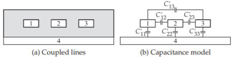
Figure \(\PageIndex{3}\): Three-line structure with four conductors labeled \(\mathsf{1, 2, 3,}\) and \(\mathsf{4}\).

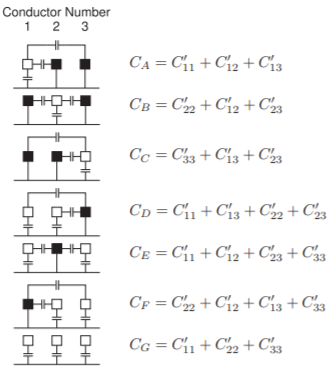
Figure \(\PageIndex{4}\): Combinations of conductors leading to various capacitance measurements. The capacitances \(C_{A},\ldots ,C_{G}\) are measured between the conductor identified by the open square and the ground that is connected to the conductors, indicated by the closed squares.

Using the first six measurements in Figure \(\PageIndex{4}\),

\[\label{eq:5}\left.\begin{array}{lll}{C_{A}=C_{11}}&{}&{C_{D} = C_{11} + 2C_{12} + C_{22}}\\{C_{B}=C_{22}}&{}&{C_{E} = C_{11} + 2C_{13} + C_{33}}\\{C_{C}=C_{33}}&{}&{C_{F} = C_{22} + 2C_{23} + C_{33}}\end{array}\right\} \]

Thus

\[\label{eq:6}\left.\begin{array}{lll}{C_{11}=C_{A}}&{}&{C_{12} = C_{21} =\frac{1}{2} (C_{D} − C_{A} − C_{B})}\\{C_{22}=C_{B}}&{}&{C_{13} = C_{31} =\frac{1}{2}(C_{E} − C_{A} − C_{C} )}\\{C_{33}=C_{C}}&{}&{C_{23} = C_{32} =\frac{1}{2}(C_{F} − C_{B} − C_{C})}\end{array}\right\} \]

This extraction does not require the widths of the strips to be the same.