6.3: Parallel-Plate Waveguide

This section derives the propagating EM fields for the parallel-plate waveguide shown in Figure \(\PageIndex{1}\). The parallel-plate waveguide shown in Figure \(\PageIndex{1}\)(a) has conducting planes at the top and bottom that (as an approximation) extend infinitely in the \(x\) direction. Electromagnetic fields introduced between the plates, say by a sinusoidally varying voltage generator across the plates, will be guided by the charges and currents induced in the conductors.

The parallel-plate waveguide structure occurs in many planar circuits, such as between the ground and power planes of circuit boards. Understanding the EM propagation supported by parallel-plate waveguides enables design choices to be made that suppress unwanted propagation modes.

6.3.1 TEM Mode

In the transverse EM (TEM) mode, all of the \(E\) and \(H\) field components are in the plane transverse to the direction of propagation, that is, \(E_{z} =0= H_{z}\). Thus Equation (6.2.26) requires that \(E_{x},\: E_{y},\: H_{x},\) and \(H_{y}\) cannot vary with position in the transverse plane (i.e., with respect to \(x\) and \(y\)). Thus \(E_{x},\: E_{y},\: H_{x},\) and \(H_{y}\) must be constant between the plates. Furthermore, boundary conditions require that \(H_{y} = 0\) and \(E_{x} = 0\) at the conductors. So in the TEM parallel-plate mode, only \(E_{y}\) and \(H_{x}\) exist, and they are constant. Equation

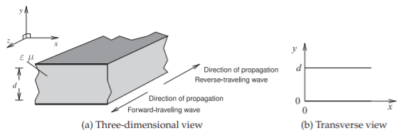
Figure \(\PageIndex{1}\): Parallel-plate waveguide.

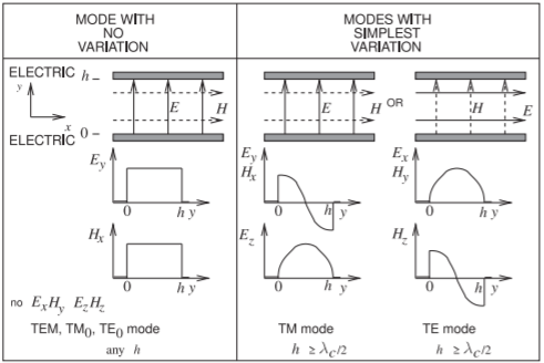
Figure \(\PageIndex{2}\): Lowest-order modes supported by combinations of electric and magnetic walls for the TEM \((=\text{TM}_{0} = \text{TE}_{0})\), \(\text{TM}_{1}\), and \(\text{TE}_{1}\) modes.

(6.2.25) leads to

\[\label{eq:1}H_{x}=\frac{\gamma E_{y}}{\jmath\omega\mu}=\pm\frac{\jmath\omega\sqrt{\mu\varepsilon}}{\jmath\omega\mu}E_{y}=\pm\sqrt{\frac{\varepsilon}{\mu}}E_{y}=\pm\frac{1}{\eta}E_{y} \]

where the plus sign describes forward-traveling fields (propagating in the \(+z\) direction) and the minus sign describes backward-traveling fields (propagating in the \(−z\) direction). The quantity \(\eta = \sqrt{\mu/\varepsilon}\) is called the wave impedance, it is the intrinsic impedance of the medium between the parallel plates. This field variation is shown on the left in Figure \(\PageIndex{2}\)(a). The TEM mode exists down to DC.

To determine the characteristic impedance of the parallel-plate waveguide first calculate the voltage of the top plate with respect to the bottom plate. This voltage is the integral of the electric field between the plates:

\[\label{eq:2}V=-\int_{y=0}^{d}E_{y}\text{e}^{-\gamma z}dy=E_{y}d\text{e}^{-\gamma z} \]

since \(E_{y}\) is a constant. The current on the top plate in the \(z\) direction is obtained by integrating the surface current density in the \(x\) direction. Assuming that the plates have a width \(W\) in the \(x\) direction then the current on the top plate is

\[\label{eq:3}I=-\int_{x=0}^{W}J_{s}\cdot\hat{z}dx=H_{x}W\text{e}^{-\jmath z} \]

since \(E_{y}\) is a constant. In terms of voltage and current (and hence treating the parallel-plate waveguide as a transmission line) the characteristic impedance of the TEM mode is

\[\label{eq:4}Z_{0}=\frac{V}{I}=\frac{E_{y}d}{H_{x}W}=\frac{\eta d}{W} \]

Here \(\eta\) is the intrinsic impedance of a TEM mode in the medium. Since we are considering a TEM mode, the wave impedance of the TEM mode is just the intrinsic impedance, that is,

\[\label{eq:5}Z_{\text{TEM}}=E_{y}/H_{x}=Z_{0}|_{\text{free-space}}=\eta \]

With \(\eta_{0} =\sqrt{\mu_{0}/\varepsilon_{0}}\) being the free-space impedance, the characteristic impedance can be written

\[\label{eq:6}Z_{0}=\frac{\eta_{0}d}{W}\sqrt{\frac{\mu_{r}}{\varepsilon_{r}}}\quad\text{and}\quad Z_{\text{TEM}}=\eta=\eta_{0}\sqrt{\frac{\mu_{r}}{\varepsilon_{r}}} \]

The phase velocity \((= \omega/\beta)\) is just the speed of light in the medium:

\[\label{eq:7}v_{p}=\frac{1}{\sqrt{\mu_{0}\varepsilon_{0}}}=\frac{c}{\sqrt{\mu_{r}\varepsilon_{r}}} \]

Formulas for attenuation are developed in [1] and the conductor attenuation

\[\label{eq:8}\alpha_{c}=\frac{R_{s}}{\eta d}\quad\text{(with SI units of Np/m)} \]

where \(R_{s} = 1/(\sigma\delta_{s})\) is the surface resistance of the conductor, \(\sigma\) is the conductivity of the conductor, and \(\delta_{s}\) is the skin depth in the conductor. The attenuation due to dielectric loss is

\[\label{eq:9}\alpha_{d}=\frac{k^{2}\tan\delta}{2\beta}\quad\text{(with SI units of Np/m)} \]

6.3.2 TM Mode

The Transverse Magnetic Mode (TM) is characterized by \(H_{z} = 0\). Another restriction that will be used here in developing the field equations is that there is no variation of the fields in the \(x\) direction. Examining Equation (6.2.25) the only components of the field that could exist are \(E_{y},\: E_{z},\) and \(H_{x}\). Everywhere \(E_{y}\) is perpendicular, and \(H_{y}\) is parallel, to the electrical walls so boundary conditions are satisfied for \(E_{y}\) and \(H_{x}\). \(E_{z}\) will be parallel to the electrical walls at the walls so boundary conditions need to be applied in deriving \(E_{z}\).

The boundary conditions are that the \(E\) field parallel to the conducting walls is zero. Considering \(E_{z}\) only, Equation (6.2.18) becomes

\[\label{eq:10}\frac{d^{2}E_{z}}{dy^{2}}=-k_{c}^{2}E_{z} \]

The solution to Equation \(\eqref{eq:10}\) is

\[\label{eq:11}E_{z}=[E_{0}\sin(k_{c}y)+E_{1}\cos(k_{c}y)]\text{e}^{-\gamma z} \]

To find the coefficients \(E_{0}\) and \(E_{1}\) boundary conditions are applied so that \(E_{z}\) is zero at \(y = 0\) and \(y = d\) (since the \(E\) field parallel to the conductors must be zero), that is,

\[\label{eq:12}E_{z}|_{y=0}=0=E_{1}\quad\text{and}\quad E_{z}|_{y=d}=0=E_{0}\sin(k_{c}d) \]

This requires that \(\sin(k_{c}d)=0\), and thus requiring that there are discrete values of \(k_{c}\):

\[\label{eq:13}k_{c}=m\pi/d\quad m=1,2,3,\ldots \]

(Note that \(m = 0\) is also a solution but requires a separate derivation, see the summary for this section.) Each value of \(k_{c}\) identifies a different mode and \(m\) is the mode index. The \(m\)th mode is the \(\text{TM}_{m}\) mode and \(m\) indicates the number of half-sinusoidal variations of the fields in the \(y\) direction. The \(\text{TM}_{m}\) mode propagates if the wavelength of the signal is such that \(\lambda ≥\lambda_{c}\), where \(\lambda_{c}\) is the critical wavelength of the \(m\)th mode

Substituting the above results and assumptions (e.g., \(\partial/\partial x = 0\)) in Equation (6.2.25),

\[\begin{align}\label{eq:14}H_{z}&=0\: E_{x}=0\: H_{y}=0 \\ \label{eq:15}E_{z}&=E_{0}\sin(k_{c}y)\text{e}^{-\gamma z} \\ \label{eq:16}E_{y}&=-\frac{\gamma}{k_{c}^{2}}\frac{dE_{z}}{dy}=-\frac{\gamma}{k_{c}}E_{0}\cos(k_{c}y)\text{e}^{-\gamma z} \\ \label{eq:17}H_{x}&=\frac{\jmath\omega\varepsilon}{k_{c}^{2}}\frac{dE_{z}}{dy}=\frac{\jmath\omega\varepsilon}{k_{c}}E_{0}\cos(k_{c}y)\text{e}^{-\gamma z}\end{align} \]

These are the complete field descriptions of the TM parallel-plate waveguide modes with zero variation in the \(x\) direction. Recall that the wavenumber \(k =\omega\sqrt{\mu\varepsilon}\).

There are an infinite number of TM modes identified by the index \(m\), which determines the cutoff wavenumber, \(k_{c}\), of the particular mode. The propagation constant of the \(m\)th mode, i.e. the \(\text{TM}_{m}\) mode, is

\[\label{eq:18}\gamma=\sqrt{k_{c}^{2}-k^{2}}=\sqrt{(m\pi/d)^{2}-\omega^{2}\mu\varepsilon} \]

Propagation is only possible if \(\gamma\) has an imaginary component. Thus in a lossless medium \(\gamma = \jmath\beta\) and \(\beta =\sqrt{k^{2}-k_{c}^{2}}\). The cutoff frequency below which propagation is not possible is

\[\label{eq:19}f_{c}=\frac{1}{2\pi}\frac{k_{c}}{\sqrt{\mu\varepsilon}}=\frac{1}{2\pi}\frac{m\pi}{d\sqrt{\mu\varepsilon}}=\frac{m\nu}{2d} \]

where \(\nu = 1/\sqrt{\mu\varepsilon}\) is the velocity of a TEM mode in the medium. The cutoff wavelength can also be defined as

\[\label{eq:20}\lambda_{c}=\frac{\nu}{f_{c}}=\frac{2d}{m} \]

where \(\nu\) is the speed of light in the medium. The wavelength of the \(\text{TM}_{m}\) mode, at a particular frequency, is the guide wavelength

\[\label{eq:21}\lambda_{g}=\frac{2\pi}{\beta}=\frac{\lambda}{\sqrt{1-(f_{c}/f)^{2}}} \]

where \(\lambda\) is the wavelength of a TEM mode in the medium: \(\lambda = \nu /f\) (so \(\lambda_{g} =\lambda\) when \(k_{c} = 0\)). The phase velocity of the modes is dependent on the mode index \(m\) through the cutoff frequency:

\[\label{eq:22}v_{p}=\frac{\omega}{\beta}=\frac{\nu}{\sqrt{1-(f_{c}/f)^{2}}} \]

and the group velocity is

\[\label{eq:23}v_{g}=\frac{d\omega}{d\beta}=\nu\sqrt{1-(f_{c}/f)^{2}} \]

The phase velocity, \(v_{p}\), of a TM mode is greater than \(\nu\) while the group velocity, \(v_{g}\), is slower than \(\nu\). The group velocity is the velocity at which energy is transmitted and thus can never be faster than the speed of light, \(c\). The phase velocity, however, can be greater than \(c\). The TM mode field variation is shown on the right in Figure \(\PageIndex{2}\).

The wave impedance of the \(\text{TM}_{m}\) mode is

\[\label{eq:24}Z_{\text{TM}}=-E_{y}/H_{x}=\frac{\beta}{\omega\varepsilon}=\frac{\beta\eta}{k} \]

Formulas for attenuation are developed in [1] and the conductor attenuation

\[\label{eq:25}\alpha_{c}=\frac{2kR_{s}}{\beta\eta d}\quad\text{(with SI units of Np/m)} \]

where \(R_{s} = 1/(\sigma\delta_{s})\) is the surface resistance of the conductor, \(\sigma\) is the conductivity of the conductor, and \(\delta_{s}\) is the skin depth in the conductor. The attenuation due to dielectric loss is

\[\label{eq:26}\alpha_{d}=\frac{k^{2}\tan\delta}{2\beta}\quad\text{(with SI units of Np/m)} \]

6.3.3 TE Mode

The transverse electric (TE) mode is characterized by \(E_{z}= 0\). Following the same development as for the TM modes, the \(\text{TE}_{n}\) mode fields with \(n\) variations of the \(H_{z}\) are

\[\begin{align}\label{eq:27}E_{z}&=0,\: E_{y}=0,\: H_{x}=0 \\ \label{eq:28}H_{z}&=H_{0}\cos(k_{c}y)\text{e}^{-\gamma z} \\ \label{eq:29}E_{x}&=\frac{\jmath\omega\mu}{k_{c}}H_{0}\sin(k_{c}y)\text{e}^{-\gamma z} \\ \label{eq:30}H_{y}&=\frac{\gamma}{k_{c}}H_{0}\sin(k_{c}y)\text{e}^{-\gamma z}\end{align} \]

The equations for \(k_{c},\: v_{p},\: v_{g},\: f_{c},\: \lambda_{c},\) and \(\lambda_{g}\) of the \(\text{TE}_{n}\) mode are the same as for the \(\text{TM}_{m}\) mode considered in the previous section with the replacement of the mode index \(m\) by \(n\), \(n = 1, 2, 3,\ldots\). (Note that \(n = 0\) is also a solution but requires a separate derivation, see the summary for this section.) The TE mode field variation is shown on the right in Figure \(\PageIndex{2}\).

The wave impedance of the TE mode is

\[\label{eq:31}Z_{\text{TE}}=\frac{k\eta}{\beta} \]

Formulas for attenuation are developed in [1] and the conductor attenuation

\[\label{eq:32}\alpha_{c}=\frac{2k_{c}^{2}R_{s}}{k\beta\eta d}\quad\text{(with SI units of Np/m)} \]

where \(R_{s} = 1/(\sigma\delta_{s})\) is the surface resistance, \(\eta\), of the conductor, \(\sigma\) is the conductivity of the conductor, and \(\delta_{s}\) is the skin depth pf the conductor. The attenuation due to dielectric loss is

\[\label{eq:33}\alpha_{d}=\frac{k^{2}\tan\delta}{2\beta}\quad\text{(with SI units of Np/m)} \]

6.3.4 Summary

The TEM mode (where \(k_{c} = 0\)) is the same as the \(\text{TM}_{0}\) mode and the \(\text{TE}_{0}\) mode. Here derivations of the TE and TM modes began with from Equation (6.2.25) and were only solutions for \(k_{c}\neq 0\). Development of the \(0th\) order TE and TM modes requires derivation from Equation (6.2.26) but this was done for the TEM mode and so was not repeated for the \(\text{TE}_{0}\) and \(\text{TM}_{0}\) modes.