6.1: Introduction

Last updated
Save as PDF

Page ID: 41063

\( \newcommand{\vecs}[1]{\overset { \scriptstyle \rightharpoonup} {\mathbf{#1}} } \) \( \newcommand{\vecd}[1]{\overset{-\!-\!\rightharpoonup}{\vphantom{a}\smash {#1}}} \)\(\newcommand{\id}{\mathrm{id}}\) \( \newcommand{\Span}{\mathrm{span}}\) \( \newcommand{\kernel}{\mathrm{null}\,}\) \( \newcommand{\range}{\mathrm{range}\,}\) \( \newcommand{\RealPart}{\mathrm{Re}}\) \( \newcommand{\ImaginaryPart}{\mathrm{Im}}\) \( \newcommand{\Argument}{\mathrm{Arg}}\) \( \newcommand{\norm}[1]{\| #1 \|}\) \( \newcommand{\inner}[2]{\langle #1, #2 \rangle}\) \( \newcommand{\Span}{\mathrm{span}}\) \(\newcommand{\id}{\mathrm{id}}\) \( \newcommand{\Span}{\mathrm{span}}\) \( \newcommand{\kernel}{\mathrm{null}\,}\) \( \newcommand{\range}{\mathrm{range}\,}\) \( \newcommand{\RealPart}{\mathrm{Re}}\) \( \newcommand{\ImaginaryPart}{\mathrm{Im}}\) \( \newcommand{\Argument}{\mathrm{Arg}}\) \( \newcommand{\norm}[1]{\| #1 \|}\) \( \newcommand{\inner}[2]{\langle #1, #2 \rangle}\) \( \newcommand{\Span}{\mathrm{span}}\)\(\newcommand{\AA}{\unicode[.8,0]{x212B}}\)

Rectangular waveguides are used to route millimeter-wave signals and high power microwave signals. The rectangular waveguide, often called just waveguide, shown in Figure \(\PageIndex{1}\) has metal walls forming a rectangular pipe. Charges and currents induced in the conductive walls guide propagating EM fields in the \(+z\) and \(−z\) directions. The rectangular waveguide has very little loss compared to a coaxial line because the EM field is away from the walls and there is little current in the walls, and what is there is spread out resulting in low current density. All of the waveguide loss, as with the loss of most transmission systems, is resistive loss so minimizing current density minimizes loss.

This chapter begins with Section 6.2 where symmetries and restricting

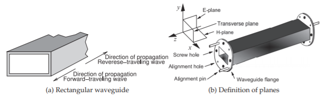
Figure \(\PageIndex{1}\): Rectangular waveguide.

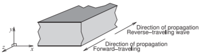
Figure \(\PageIndex{2}\): Parallel-plate waveguide.

propagation to only the \(±z\) direction are applied to Maxwell’s equations to yield the rectangular wave equation. These are then used in Section 6.3 to describe propagation between two metal planes forming what is called a parallel-plate waveguide, see Figure \(\PageIndex{2}\). Then the rectangular wave equations are applied to a rectangular waveguide in Section 6.4 to derive the field distribution inside a rectangular waveguide.