2.3: The Lowpass Filter Prototype

Last updated
Save as PDF

Page ID: 46096

\( \newcommand{\vecs}[1]{\overset { \scriptstyle \rightharpoonup} {\mathbf{#1}} } \) \( \newcommand{\vecd}[1]{\overset{-\!-\!\rightharpoonup}{\vphantom{a}\smash {#1}}} \)\(\newcommand{\id}{\mathrm{id}}\) \( \newcommand{\Span}{\mathrm{span}}\) \( \newcommand{\kernel}{\mathrm{null}\,}\) \( \newcommand{\range}{\mathrm{range}\,}\) \( \newcommand{\RealPart}{\mathrm{Re}}\) \( \newcommand{\ImaginaryPart}{\mathrm{Im}}\) \( \newcommand{\Argument}{\mathrm{Arg}}\) \( \newcommand{\norm}[1]{\| #1 \|}\) \( \newcommand{\inner}[2]{\langle #1, #2 \rangle}\) \( \newcommand{\Span}{\mathrm{span}}\) \(\newcommand{\id}{\mathrm{id}}\) \( \newcommand{\Span}{\mathrm{span}}\) \( \newcommand{\kernel}{\mathrm{null}\,}\) \( \newcommand{\range}{\mathrm{range}\,}\) \( \newcommand{\RealPart}{\mathrm{Re}}\) \( \newcommand{\ImaginaryPart}{\mathrm{Im}}\) \( \newcommand{\Argument}{\mathrm{Arg}}\) \( \newcommand{\norm}[1]{\| #1 \|}\) \( \newcommand{\inner}[2]{\langle #1, #2 \rangle}\) \( \newcommand{\Span}{\mathrm{span}}\)\(\newcommand{\AA}{\unicode[.8,0]{x212B}}\)

Most filter design is based on the synthesis of a lowpass filter equivalent called a lowpass prototype. Transformations are then used to correct for the actual source and load impedances, frequency range, and the desired filter type, such as highpass or bandpass. An ideal lowpass response is shown in Figure \(\PageIndex{1}\)(a), which shows a transmission coefficient of \(1\) up to a normalized frequency of \(1\text{ rad/sec}\). This type of response defines what is called a brick-wall filter, which unfortunately cannot be physically realized. Instead, the response is approximated and specified in terms of a response template (see Figure \(\PageIndex{1}\)(b)).

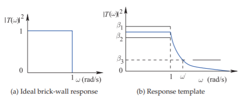
Figure \(\PageIndex{1}\): Lowpass filter response.

The template specifies a passband response that is between \(\beta_{1}\) and \(\beta_{2}\) at frequencies below the corner radian frequency (at \(\omega = 1\)), and below \(\beta_{3}\) above a radian frequency \(\omega′ > 1\). The lowpass filter is harder to realize the closer the specified response is to the ideal response shown in Figure \(\PageIndex{1}\)(a), that is, when

\[\label{eq:1}(\beta_{2}-\beta_{1})\to 0,\quad\beta_{3}\to 0,\quad\text{and}\quad (\omega '-1)\to 0 \]

Several polynomials have particularly interesting characteristics that match the requirements of the response template. At first it may seem surprising that polynomial functions could yield close to ideal filter responses. However, as will be seen, there is something special about these polynomials: they are natural solutions to extreme conditions. For example, the \(n\)th-order Butterworth polynomial has the special property that the first \(n\) derivatives at \(s = 0\) are zero. The other polynomials also have extreme properties, and filters that are synthesized using them also have extreme properties. As well as the maximally flat property resulting from Butterworth polynomials, filter responses obtained using Chebyshev polynomials have the steepest skirts (i.e., fastest transitions from the frequency region where signals are passed to the region where they are blocked). Usually it is one of these extreme cases that is most desirable.

A streamlining of the filter synthesis procedure is obtained by first focusing on the development of normalized lowpass filters having a \(1\text{ rad/s}\) corner frequency and \(1\:\Omega\) reference impedance. Transformations transform a lowpass filter prototype into another filter having the response desired. These transformations give rise to symmetrical responses.