
2.7: Butterworth and Chebyshev Filters
- Page ID
- 46103
The \(n\)th-order lowpass filters constructed from the Butterworth and Chebyshev polynomials have the ladder circuit forms of Figure \(\PageIndex{1}\)(a or b). Figure \(\PageIndex{1}\) uses several shorthand notations commonly used with filters. First, note that there are two prototype forms designated Type \(1\) and Type \(2\), and these are referred to as duals of each other. The two prototype forms have identical responses with the same numerical element values \(g_{1},\ldots , g_{n}\). Consider the Type \(1\) prototype of Figure \(\PageIndex{1}\)(a). The right-most element is the resistive load, which is also known as the \((n + 1)\)th element. The next element to the left of this is either a shunt capacitor (of value \(g_{n}\)) if \(n\) is even, or a series inductor (of value \(g_{n}\)) if \(n\) is odd. So for the Type \(1\) prototype, the shunt capacitor next to the load does not exist if \(n\) is odd. The same interpretation applies to the circuit in Figure \(\PageIndex{1}\)(b).
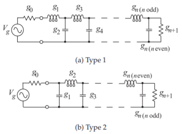
Figure \(\PageIndex{1}\): Filter prototypes in the Cauer topology. Here \(n\) is the order of the filter.
| Order, \(n\) | \(2\) | \(3\) | \(4\) | \(5\) | \(6\) | \(7\) | \(8\) | \(9\) |
|---|---|---|---|---|---|---|---|---|
| \(g_{1}\) | \(1.4142\) | \(1\) | \(0.7654\) | \(0.6180\) | \(0.5176\) | \(0.4450\) | \(0.3902\) | \(0.3473\) |
| \(g_{2}\) | \(1.4142\) | \(2\) | \(1.8478\) | \(1.6180\) | \(1.4142\) | \(1.2470\) | \(1.1111\) | \(1\) |
| \(g_{3}\) | \(1\) | \(1\) | \(1.8478\) | \(2\) | \(1.9318\) | \(1.8019\) | \(1.6629\) | \(1.5321\) |
| \(g_{4}\) | \(1\) | \(0.7654\) | \(1.6180\) | \(1.9318\) | \(2\) | \(1.9615\) | \(1.8794\) | |
| \(g_{5}\) | \(1\) | \(0.6180\) | \(1.4142\) | \(1.8019\) | \(1.9615\) | \(2\) | ||
| \(g_{6}\) | \(1\) | \(0.5176\) | \(1.2470\) | \(1.6629\) | \(1.8794\) | |||
| \(g_{7}\) | \(1\) | \(0.4450\) | \(1.1111\) | \(1.5321\) | ||||
| \(g_{8}\) | \(1\) | \(0.3902\) | \(1\) | |||||
| \(g_{9}\) | \(1\) | \(0.3473\) | ||||||
| \(g_{10}\) | \(1\) |
Table \(\PageIndex{1}\): Coefficients of the Butterworth lowpass prototype filter normalized to a radian corner frequency of \(1\text{ rad/s}\) and a \(1\:\Omega\) system impedance (i.e., \(g_{0} =1= g_{n+1}\)).
2.7.1 Butterworth Filter
A generalization of the example of the previous section leads to a formula for the element values of a ladder circuit implementing a Butterworth lowpass filter. For a maximally flat or Butterworth response the element values of the circuit in Figure \(\PageIndex{1}\)(a and b) are
\[\label{eq:1}g_{r}=2\sin\left\{ (2r-1)\frac{\pi}{2n}\right\}\quad r=1,2,3,\ldots ,n \]
and \(g_{0} =1= g_{n+1}\). Table \(\PageIndex{1}\) lists the coefficients of Butterworth lowpass prototype filters up to ninth order.
Example \(\PageIndex{1}\): Fourth-Order Butterworth Lowpass Filter
Derive the fourth-order Butterworth lowpass prototype of Type \(1\).
Solution
From Equation \(\eqref{eq:1}\),
\[\begin{align}\label{eq:2} g_{1}&=2\sin [\pi /(2\cdot 4)]=0.765369\text{ H} \\ \label{eq:3} g_{2}&=2\sin [3\pi /(2\cdot 4)]=1.847759\text{ F} \\ \label{eq:4} g_{3}&=2\sin [5\pi /(2\cdot 4)]=1.847759\text{ H} \\ \label{eq:5} g_{4}&=2\sin [7\pi /(2\cdot 4)]= 0.765369\text{ F}\end{align} \]
Thus the fourth-order Butterworth lowpass prototype circuit with a corner frequency of \(1\text{ rad/s}\) is as shown in Figure \(\PageIndex{2}\).
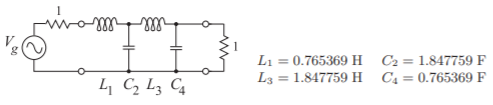
Figure \(\PageIndex{2}\): Fourthorder Butterworth lowpass filter prototype.
2.7.2 Chebyshev Filter
For a Chebyshev response, the element values of the lowpass prototype shown in Figure \(\PageIndex{1}\) are found from the recursive formula [1, 6, 7]:
\[\begin{align}\label{eq:6} g_{0}&=1\quad g_{1}=\frac{2a_{1}}{\gamma} \\ \label{eq:7} g_{n+1}&=\left\{\begin{array}{ll}{1}&{n\text{ odd}} \\ {\tanh^{2}(\beta /4)}&{n\text{ even}}\end{array}\right\} \\ \label{eq:8}g_{k}&=\frac{4a_{k-1}a_{k}}{b_{k-1}g_{k-1}},\quad k=1,2,\ldots ,n \\ \label{eq:9}a_{k}&=\sin\left[\frac{(2k-1)\pi}{2n}\right]\quad k=1,2,\ldots ,n\end{align} \]
where
\[\begin{align}\label{eq:10}\gamma&=\sinh\left(\frac{\beta}{2n}\right) \\ \label{eq:11} b_{k}&=\gamma^{2}+\sin^{2}\left(\frac{k\pi}{n}\right)\quad k=1,2,\ldots ,n \\ \label{eq:12}\beta &=\ln\left[\coth\left(\frac{R_{\text{dB}}}{2\cdot 20\log(2)}\right)\right] = \ln\left[\coth\left(\frac{R_{\text{dB}}}{17.3717793}\right)\right] \\ \label{eq:13}R_{\text{dB}}&=10\log(1+\varepsilon^{2})\end{align} \]
\(n\) is the order of the filter, and \(\varepsilon\) is the ripple factor and defines the level of the ripple in absolute terms. \(R_{\text{dB}}\) is the ripple expressed in decibels (the ripple is generally specified in decibels).
An interesting point to note here is that the source resistor, the value of which is given by \(g_{0}\), and terminating resistor, the value of which is given by \(g_{n+1}\), are only equal for odd-order filters. For an even-order Chebyshev filter the terminating resistor, \(g_{n+1}\), will be different and a function of the filter ripple. Because it is generally desirable to have identical source and load impedances, Chebyshev filters are nearly always restricted to odd order. Thus the odd-order Chebyshev prototypes are as shown in Figure \(\PageIndex{3}\).
Also, for an odd-degree function (\(n\) is odd) there is a perfect match at DC,
\[\label{eq:14}|T(0)|^{2}=1 \]
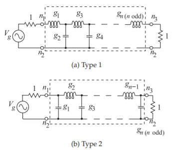
Figure \(\PageIndex{3}\): Odd-order Chebyshev lowpass filter prototypes in the Cauer topology. Here \(n\) is the order of the filter.
| Order Ripple | \(n=3\) | |||||
|---|---|---|---|---|---|---|
| \(0.01\text{ dB}\) | \(0.1\text{ dB}\) | \(0.2\text{ dB}\) | \(1.0\text{ dB}\) | \(3.0\text{ dB}\) | \(\varepsilon =0.1\) | |
| \(g_{1}\) | \(0.62918\) | \(1.03156\) | \(1.22754\) | \(2.02359\) | \(3.34874\) | \(0.85158\) |
| \(g_{2}\) | \(0.97028\) | \(1.14740\) | \(1.15254\) | \(0.99410\) | \(0.71170\) | \(1.10316\) |
| \(g_{3}\) | \(0.62918\) | \(1.03156\) | \(1.22754\) | \(2.02359\) | \(3.34874\) | \(0.85158\) |
| Order Ripple | \(n=5\) | |||||
| \(0.01\text{ dB}\) | \(0.1\text{ dB}\) | \(0.2\text{ dB}\) | \(1.0\text{ dB}\) | \(3.0\text{ dB}\) | \(\varepsilon =0.1\) | |
| \(g_{1}\) | \(0.75633\) | \(1.14681\) | \(1.33944\) | \(2.13488\) | \(3.48129\) | \(0.97140\) |
| \(g_{2}\) | \(1.30492\) | \(1.37121\) | \(1.33702\) | \(1.09111\) | \(0.76192\) | \(1.37208\) |
| \(g_{3}\) | \(1.57731\) | \(1.97500\) | \(2.16605\) | \(3.00092\) | \(4.53755\) | \(1.80136\) |
| \(g_{4}\) | \(1.30492\) | \(1.37121\) | \(1.33702\) | \(1.09111\) | \(0.76192\) | \(1.37208\) |
| \(g_{5}\) | \(0.75633\) | \(1.14681\) | \(1.33944\) | \(2.13488\) | \(3.48129\) | \(0.97140\) |
| Order Ripple | \(n=7\) | |||||
| \(0.01\text{ dB}\) | \(0.1\text{ dB}\) | \(0.2\text{ dB}\) | \(1.0\text{ dB}\) | \(3.0\text{ dB}\) | \(\varepsilon =0.1\) | |
| \(g_{1}\) | \(0.79694\) | \(1.18118\) | \(1.37226\) | \(2.16656\) | \(3.51852\) | \(1.00794\) |
| \(g_{2}\) | \(1.39242\) | \(1.42281\) | \(1.37820\) | \(1.11151\) | \(0.77220\) | \(1.43678\) |
| \(g_{3}\) | \(1.74813\) | \(2.09667\) | \(2.27566\) | \(3.09364\) | \(4.63898\) | \(1.93981\) |
| \(g_{4}\) | \(1.63313\) | \(1.57340\) | \(1.50016\) | \(1.17352\) | \(0.80381\) | \(1.62196\) |
| \(g_{5}\) | \(1.74813\) | \(2.09667\) | \(2.27566\) | \(3.09364\) | \(4.63898\) | \(1.93981\) |
| \(g_{6}\) | \(1.39242\) | \(1.42281\) | \(1.37820\) | \(1.11151\) | \(0.77220\) | \(1.43678\) |
| \(g_{7}\) | \(0.79694\) | \(1.18118\) | \(1.37226\) | \(2.16656\) | \(3.51852\) | \(1.00794\) |
| Order Ripple | \(n=9\) | |||||
| \(0.01\text{ dB}\) | \(0.1\text{ dB}\) | \(0.2\text{ dB}\) | \(1.0\text{ dB}\) | \(3.0\text{ dB}\) | \(\varepsilon =0.1\) | |
| \(g_{1}\) | \(0.81446\) | \(1.19567\) | \(1.38603\) | \(2.17972\) | \(3.53394\) | \(1.02347\) |
| \(g_{2}\) | \(1.42706\) | \(1.44260\) | \(1.39389\) | \(1.11918\) | \(0.76604\) | \(1.46186\) |
| \(g_{3}\) | \(1.80436\) | \(2.13455\) | \(2.30932\) | \(3.12143\) | \(4.66906\) | \(1.98372\) |
| \(g_{4}\) | \(1.71254\) | \(1.61672\) | \(1.53405\) | \(1.18967\) | \(0.81181\) | \(1.67776\) |
| \(g_{5}\) | \(1.90579\) | \(2.20537\) | \(2.37280\) | \(3.17463\) | \(4.72701\) | \(2.06485\) |
| \(g_{6}\) | \(1.71254\) | \(1.61672\) | \(1.53405\) | \(1.18967\) | \(0.81181\) | \(1.67776\) |
| \(g_{7}\) | \(1.80436\) | \(2.13455\) | \(2.30932\) | \(3.12143\) | \(4.66906\) | \(1.98372\) |
| \(g_{8}\) | \(1.42706\) | \(1.44260\) | \(1.39389\) | \(1.11918\) | \(0.76604\) | \(1.46186\) |
| \(g_{9}\) | \(0.81446\) | \(1.19567\) | \(1.38603\) | \(2.17972\) | \(3.53394\) | \(1.02347\) |
Table \(\PageIndex{2}\): Coefficients of a Chebyshev lowpass prototype filter normalized to a radian corner frequency of \(\omega_{0} = 1\text{ rad/s}\) and a \(1\:\Omega\) system impedance (i.e., \(g_{0} = 1 = g_{n+1}\)). The ripple factor, \(\varepsilon\), is related to the ripple in decibels by Equation \(\eqref{eq:13}\) (e.g., \(\varepsilon = 0.1\) is a ripple of \(0.0432\text{ dB}\)). (Note that \(\omega_{0}\) is the radian frequency at which the transmission response of a Chebyshev filter is down by the ripple, see Figure 2.4.2.)
while for an even-degree function (i.e., \(n\) is even) a mismatch exists of value
\[\label{eq:15}|T(0)|^{2}=\frac{4R_{L}}{(R_{L}+1)^{2}}=\frac{1}{1+\varepsilon^{2}} \]
so that
\[\label{eq:16}R_{L}=g_{n+1}=\left[\varepsilon +\sqrt{(1+\varepsilon^{2})}\right]^{2} \]
Coefficients of several Chebyshev lowpass prototype filters with different levels of ripple and odd orders up to ninth order are given in Table \(\PageIndex{2}\).
2.7.3 Summary
A Butterworth filter has a monotonic response without ripple, but a relatively slow transition from the passband to the stopband. A Chebyshev filter has a rapid transition but has ripple in either the stopband or passband. Butterworth and Chebyshev filters are special cases of elliptical filters, which are also called Cauer filters. In general, an elliptical filter has ripple in both the stopband and the passband. The level of the ripple can be selected
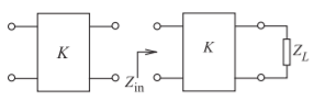
Figure \(\PageIndex{4}\): Impedance inverter (of impedance K in ohms): (a) represented as a two-port; and (b) the two-port terminated in a load.
independently in each band. With zero ripple in the stopband, but ripple in the passband, an elliptical filter becomes a Type I Chebyshev filter. With zero ripple in the passband, but ripple in the stopband, an elliptical filter becomes a Type II Chebyshev filter. With no ripple in either band the elliptical filter becomes a Butterworth filter. With ripple in both the passband and stopband, the transition between the passband and stopband can be made more abrupt or alternatively the tolerance to component variations increased.
Another type of filter is the Bessel filter which has maximally flat group delay in the passband, which means that the phase response has maximum linearity across the passband. The Legendre filter (also known as the optimum “L” filter) has a high transition rate from passband to stopband for a given filter order, and also has a monotonic frequency response (i.e., without ripple). It is a compromise between the Butterworth filter, with monotonic frequency response but slower transition and the Chebyshev filter, which has a faster transition but ripples in the frequency response.
More in-depth discussions of a large class of filters along with coefficient tables and coefficient formulas are available in Matthaei et al. [1], Hunter [3], Daniels [8], Lutovac et al. [9], and in most other books dedicated solely to microwave filters.