2.9: Filter Transformations

So far the discussion has centered around lowpass filters. Filter design technology has developed so that the design of a corresponding lowpass filter is the essential first step, and this is used as a prototype to derive a filter with other characteristics. The three most important transformations are listed here:

1. Impedance scaling: A lowpass filter prototype is referenced to a standard impedance. Usually \(1\:\Omega\) is used, so the reference source and load resistances are also \(1\:\Omega\). To reference to a higher or lower impedance, scaling of the impedance of all elements of the filter is required.
2. Corner frequency scaling: The corner frequency of a lowpass filter prototype is normalized to \(1\text{ rad/s}\). To reference to another frequency, the values of the elements must be altered so that they have the same impedance at the scaled frequency.
3. Filter type transformation: These transformations enable the circuit of a lowpass filter to be converted to a circuit with a bandpass, bandstop, or highpass response. The concept is that the response at DC is to be replicated at infinite frequency for the highpass (so capacitors become inductors, etc.); to be replicated at the center of the passband for a bandpass filter (so capacitors become a shunt \(LC\) circuit); and to be inverted at the center of a bandstop filter (so capacitors become a series \(LC\) circuit).

The transformations can be performed in any order. The key point is that the complexity of the lowpass circuit design is minimal since the number of elements does not grow until the filter type transformation is performed, so this step is often done last.

2.9.1 Impedance Transformation

The lowpass prototypes discussed up to now have been referred to a \(1\:\Omega\) system. The system impedance can be changed to any level by simply scaling the impedances of all the circuit elements in a filter by the same amount, as shown in Figure \(\PageIndex{1}\). The impedance transformation follows the same procedure for all filter types (the procedure is the same for lowpass, highpass, bandpass, and bandstop filters, for example). It should also be noted that impedance scaling of a transmission line is simply multiplication of the line’s characteristic impedance by the scale factor.

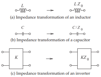
Figure \(\PageIndex{1}\): Impedance transformations. The impedances of the elements are increased by a factor \(Z_{0}\).

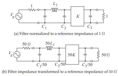
Figure \(\PageIndex{2}\): Impedance transformation of an example filter.

Example \(\PageIndex{1}\): Lowpass Filter Design

Consider the lowpass filter, with an inverter, shown in Figure \(\PageIndex{2}\)(a). This filter is referenced to \(1\:\Omega\), as the source and load impedances are both \(1\:\Omega\). Redesign the filter so that the same frequency response is obtained with \(50\:\Omega\) source and load impedances.

Solution

It is necessary to impedance transform from \(1\:\Omega\) to \(50\:\Omega\). The resulting filter is shown in Figure \(\PageIndex{2}\)(b). Each element has an impedance (resistance or reactance) that is \(50\) times larger than it had in the \(1\:\Omega\) prototype.

2.9.2 Frequency Transformation: Lowpass

Frequency transformations differ depending on the type of the filter. So it is normal to frequency transform the lowpass prototype before converting the prototype to another form (such as bandpass). The lowpass prototypes normally have a band-edge or cutoff frequency at an angular frequency of unity, that is, \(1\text{ rad/s}\). The band-edge frequency can be transformed from unity to an arbitrary angular frequency \(\omega_{c}\), as shown in Figure \(\PageIndex{3}\), by scaling the reactive elements, as shown in Figures \(\PageIndex{4}\) and \(\PageIndex{5}\)(a), so that

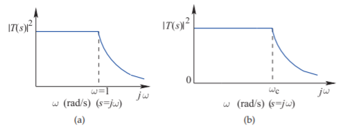
Figure \(\PageIndex{3}\): Frequency transformation of a lowpass filter response from (a) one normalized to a corner frequency of \(1\text{ rad/s}\), to (b) one with a radian corner frequency of \(\omega_{c}\).

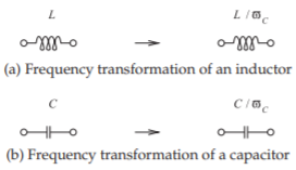
Figure \(\PageIndex{4}\): Frequency transformations. The impedance of the new (scaled) element at the new (scaled) frequency is the same as it was at the original frequency.

they have the same impedance at the transformed frequency as they did at the original frequency. The inverter is unchanged, as are the source and load resistances, since these are frequency independent.

2.9.3 Lowpass to Highpass Transformation

The transformation of a lowpass filter prototype to a highpass filter is shown diagrammatically in Figure \(\PageIndex{6}\). Mathematically \(\omega\) in the transfer function of the lowpass prototype is replaced by \(−1/\omega\), that is

\[\label{eq:1}T_{\text{highpass}}(\omega)=T_{\text{lowpass}}(-1/\omega) \]

In terms of a lumped element in the lowpass prototype circuit, if an element has an impedance \(\jmath\omega L\) and \(L\) is frequency independent, then the corresponding element in the highpass prototype filter has an impedance \(1/(\jmath\omega^{2} L)\). Thus reactive elements are transformed as shown in Figure \(\PageIndex{5}\)(b), where \(\omega_{0}\) is the corner frequency of both the lowpass and highpass prototype circuits. So inductors are transformed into capacitors and capacitors into inductors. For example, the odd-order lowpass filter prototypes shown in Figure 2.7.3 are transformed into the highpass filters shown in Figure \(\PageIndex{7}\).

2.9.4 Lowpass to Bandpass Transformation

Understanding the transformation of the lowpass filter into its corresponding bandpass form requires that the lowpass filter be considered with both its positive and negative frequency responses, as shown in Figure \(\PageIndex{8}\)(a). This response is shifted in frequency to obtain the bandpass response shown in Figure \(\PageIndex{8}\)(b). Mathematically the radian frequency, \(\omega\), in the response

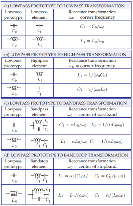
Figure \(\PageIndex{5}\): Transformations of the elements of a prototype lowpass filter to obtain specific filter types. The corner frequency of the lowpass prototype is \(1\text{ rad/s}\). In the transformations to bandpass and bandstop filters, \(\omega_{0} = 1/\sqrt{L_{1}C_{1}} = \sqrt{\omega_{1}\omega_{2}}\); \(\omega_{1}\) and \(\omega_{2}\) are the band-edge frequencies, and \(\alpha\) is the transformation constant, \(\alpha = \omega_{0}/(\omega_{2} −\omega_{1})\).

Figure \(\PageIndex{6}\): Lowpass to highpass transformation.

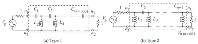
Figure \(\PageIndex{7}\): Odd-order Chebyshev highpass filter prototypes in the Cauer topology. Here n is the order of the filter.

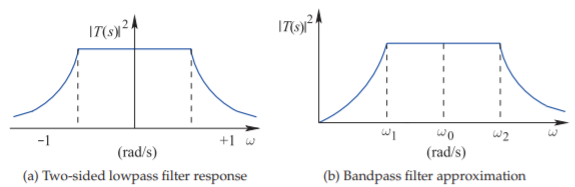
Figure \(\PageIndex{8}\): Frequency responses in lowpass to bandpass transformation \((s =\jmath\omega)\).

function is replaced by its bandpass form,

\[\label{eq:2}\omega\to\left[\frac{\omega}{\omega_{0}}-\frac{\omega_{0}}{\omega}\right] \]

That is,

\[\label{eq:3}T_{\text{bandpass}}(\omega)=T_{\text{lowpass}}\left(\frac{\omega}{\omega_{0}}-\frac{\omega_{0}}{\omega}\right) \]

and so the transfer function of the bandpass filter is derived from the transfer function of the bandpass filter with \(\omega\) replaced by \((\omega /\omega_{0} −\omega_{0}/\omega )\). This separately maps the \(−1\) and \(+1\) band-edge radian frequencies of the lowpass response to the bandpass frequencies \(\omega_{1}\) and \(\omega_{2}\):

\[\label{eq:4}-1\to\left[\frac{\omega_{1}}{\omega_{0}}-\frac{\omega_{0}}{\omega_{1}}\right]\quad\text{and}\quad +1\to\left[\frac{\omega_{2}}{\omega_{0}}-\frac{\omega_{0}}{\omega_{2}}\right] \]

Solving the above equations simultaneously yields the center frequency ω0 and the band-edge frequencies \(\omega_{1}\) and \(\omega_{2}\) with

\[\label{eq:5}\omega_{0}=\sqrt{\omega_{1}\omega_{2}} \]

and the so-called transformation constant

\[\label{eq:6}\alpha=\frac{\omega_{0}}{\omega_{2}-\omega_{1}} \]

The resulting element conversions are given in Figure \(\PageIndex{5}\)(c).

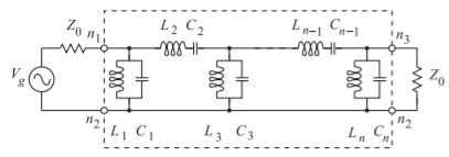
Figure \(\PageIndex{9}\): Lumped-element odd-order (\(n\)th-order) Chebyshev bandpass filter prototypes in the Type II Cauer topology.

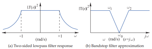
Figure \(\PageIndex{10}\): Frequency responses in lowpass to bandstop transformation.

As an example, a lumped-element Type 2 Cauer bandpass filter is shown in Figure \(\PageIndex{9}\). The shunt \(LC\) combination and the series \(LC\) combinations are resonators resonant at the center frequency of the filter. Here the filter is normalized to \(Z_{0}\) source and load impedances. As these are the same, this filter topology only applies for an odd-order filter. Combining transformations, the element values of a lumped bandpass filter with center radian frequency \(\omega_{0} = 2\pi f_{0}\) and radian bandwidth \(\omega_{\text{BW}} = 2\pi (f_{2} − f_{1})\) are as follows (\(g_{r}\) is from the lowpass prototype):

\[\label{eq:7} C_{r}=\left\{\begin{array}{ll}{\frac{g_{r}}{\omega_{\text{BW}}Z_{0}}}&{r=\text{odd}} \\ {\frac{\omega_{\text{BW}}}{\omega_{0}^{2}g_{r}Z_{0}}}&{r=\text{even}}\end{array} \right. \quad\text{and}\quad L_{r}= \left\{\begin{array}{ll}{\frac{\omega_{\text{BW}}Z_{0}}{\omega_{0}^{2}g_{r}}}&{r=\text{odd}}\\{\frac{g_{r}Z_{0}}{\omega_{\text{BW}}}}&{r=\text{even}}\end{array} \right. \]

2.9.5 Lowpass to Bandstop Transformation

Again, consider both the positive and negative frequency responses of the lowpass filter prototype, as shown in Figure \(\PageIndex{10}\)(a). This response is shifted in frequency to obtain the bandstop response shown in Figure \(\PageIndex{10}\)(b). Mathematically the frequency, \(\omega\), in the response function is replaced by its bandstop form:

\[\label{eq:8}\omega\to\left[\alpha\left(\frac{\omega}{\omega_{0}}-\frac{\omega_{0}}{\omega}\right)\right]^{-1} \]

That is,

\[\label{eq:9}T_{\text{bandstop}}(\omega)=T_{\text{lowpass}}\left(\frac{1}{\alpha}\left[\frac{\omega}{\omega_{0}}-\frac{\omega_{0}}{\omega}\right]^{-1}\right) \]

The center frequency (corresponding to DC in the lowpass prototype response) is

\[\label{eq:10}\omega_{0}=\sqrt{\omega_{1}\omega_{2}} \]

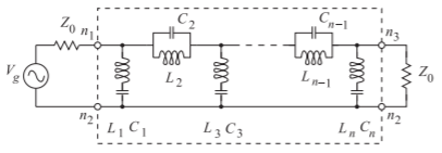
Figure \(\PageIndex{11}\): Lumped-element odd-order (\(n\)th-order) Chebyshev bandstop filter prototypes in the type II Cauer topology.

and the transformation constant is

\[\label{eq:11}\alpha=\frac{\omega_{0}}{\omega_{2}-\omega_{1}} \]

where \(\omega_{1}\) and \(\omega_{2}\) are the band-edge radian frequencies. The resulting element conversions are given in Figure \(\PageIndex{5}\)(d).

Combining transformations, the element values of a lumped bandstop filter with center radian frequency \(\omega_{0} = 2\pi f_{0}\) and radian bandwidth \(\omega_{\text{BW}} = 2\pi (f_{2} − f_{1})\) are as follows:

\[\label{eq:12}C_{r}=\left\{\begin{array}{ll}{\frac{g_{r}\omega_{\text{BW}}}{\omega_{0}^{2}Z_{0}}}&{r=\text{odd}} \\ {\frac{1}{\omega_{\text{BW}}g_{r}Z_{0}}}&{r=\text{even}}\end{array}\right.\quad\text{and}\quad L_{r}=\left\{\begin{array}{ll}{\frac{Z_{0}}{\omega_{\text{BW}}g_{r}}}&{r=\text{odd}}\\{\frac{g_{r}\omega_{\text{BW}}Z_{0}}{\omega_{0}^{2}}}&{r=\text{even}}\end{array}\right. \]

A lumped-element type II Cauer bandstop filter is shown in Figure \(\PageIndex{11}\). The parallel \(LC\) combination and the series \(LC\) combinations are resonators resonant at the center frequency of the filter. The parallel \(LC\) resonator is an open circuit at the center frequency of the stopband and the series \(LC\) resonators are short circuits. The \(LC\) resonators are implemented using resonators, usually transmission line segments and not lumped components.

2.9.6 Transformed Ladder Prototypes

Combining the filter type transformations, and with appropriate use of inverters, the original lowpass prototype ladder filter and its various filter type transforms are shown in Figure 2.10.1.