2.11: Butterworth and Chebyshev Bandpass Filters

Designs of Butterworth and Chebyshev filters with center frequencies of \(1\text{ GHz}\) and \(3\text{ dB}\) bandwidths of \(10\%\) are shown in Figure 2.10.4. Their transmission, \(S_{21}\), and reflection, \(S_{11}\), responses are shown in Figure \(\PageIndex{1}\). The filter skirts, i.e. the transitions from the passband to the stopbands, is steeper for the Chebyshev filter than for the Butterworth filter as expected. The ripple of the Chebyshev filter is very small and not seen in this plot. In a real filter there will be loss and low-level ripples in the magnitude response

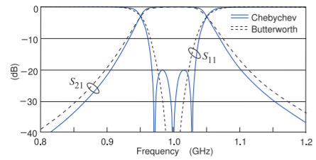
Figure \(\PageIndex{1}\): Insertion loss \((S_{21})\) and return loss \((S_{11})\) of the Butterworth and Chebychev lumped-element bandpass filters in a \(50\:\Omega\) system.

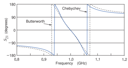
Figure \(\PageIndex{2}\): Phase of the transmission response \((S_{21})\) of the Butterworth and Chebyshev lumped-element filters. The discontinuities seen in the phase from \(−180^{\circ}\) to \(+180^{\circ}\) are artifacts and the phases of the filters reduce monotonically with increasing frequency. (For example, the phase at \(0.8\text{ GHz}\) is \(−110^{\circ} + 360^{\circ} = 250^{\circ}\).)

disappear. However even with loss the steep skirts of the Chebyshev transmission response remain. Also, even with loss, the impact of the Chebyshev ripples is clearly seen in the reflection \((S_{11})\) response. In Figure \(\PageIndex{1}\) three distinct \(S_{11}\) zeros are seen and these correspond to the three poles of the Chebyshev filter’s \(S_{21}\) response, but of course we cannot see these. (In the Laplace transfer function there are \(3\) complex poles each pair being transformed from one of the three poles of the lowpass prototype.) The Butterworth filter also has three (complex) \(S_{11}\) zeros and these are all at the center frequency of the bandpass filter, \(1\text{ GHz}\).

Another characteristic that differs between the Chebyshev and Butterworth responses is seen in their phase responses plotted in Figure \(\PageIndex{2}\). Each pole in the \(S_{21}\) characteristic causes a \(90^{\circ}\) phase change. The three complex poles (i.e. six actual poles) of \(S_{21}\) then result in six \(90^{\circ}\) phase changes in \(S_{21}\) for a total phase change of \(450^{\circ}\). Small ripples are seen in the Chebyshev phase responses in the pass band while the phase changes for the Butterworth filter are smooth. (The Chebyshev phase ripples remain even with low-level loss.)

The magnitude and phase responses, Figures \(\PageIndex{1}\) and \(\PageIndex{2}\), do not provide complete visualization of the filter characteristics. Additional insight is provided in the \(S_{11}\) loci on the Smith chart, see Figure \(\PageIndex{3}\). Figure \(\PageIndex{3}\) shows the \(S_{11}\) characteristics plotted on Smith charts. (In the passband the \(S_{21}\) locus would be very close to the unit circle and little of value is observed in the passband.) There is a wealth of information here. First consider the response for the Chebyshev filter, Figure \(\PageIndex{3}\)(a). As frequency increases from \(0.8\text{ GHz}\), the locus of \(S_{11}\) is first close to the unit circle and then approaches the origin

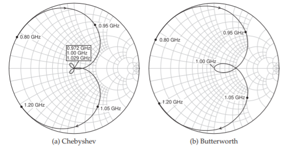
Figure \(\PageIndex{3}\): Smith chart plot of \(S_{11}\) of the Butterworth and Chebychev lumped-element filters.

of the polar plot as the frequency approaches the passband of the filter. A special characteristic of the Chebyshev response is the looping which here results in three passes of the locus through the origin. These are the three zeros. Eventually the locus of \(S_{11}\) increases as frequency increases above the passband. A loop is also seen in the Butterworth response, Figure \(\PageIndex{3}\)(b). This loop goes through the origin and while it seems that there is just one zero there are actually three. What is happening is that as frequency increases and as the locus of the Butterworth \(S_{11}\) response approaches the origin, the movement of the locus with respect to frequency slows down. The best way to be convinced that there are three zeros of \(S_{11}\) is to look at the transmission phase \((\angle S_{21})\) response in Figure \(\PageIndex{1}\).

Comprehensive visualization of the filter response requires the rectangular plots of the magnitudes of \(S_{21}\) and \(S_{11}\), Figure \(\PageIndex{1}\), of \(S_{21}\) phase, Figure \(\PageIndex{2}\), and the Smith chart plot of \(S_{11}\), Figure \(\PageIndex{3}\). The phase plot convinces you of the number of zeros in your design which is important in interpreting the Butterworth results. A physical implementation of the design will not be exact and so tuning is required. Then the most important characterizations are the rectangular magnitude and Smith chart responses. Here the loops on the Smith chart, even if they do not go through the origin exactly, distinguish the Butterworth and Chebyshev responses. Matching may be required to shift the loops to the origin of the polar plot.