3.8: Exercises

1. A parallel coupled-line section is shown in Figure 3.2.11. The even-mode impedance of the coupled line is \(60\:\Omega\) and the odd-mode impedance is \(40\:\Omega\). The PCL section is \(\lambda/4\) long at the center frequency of the section.
   1. What is the system impedance \(Z_{0S}\)?
   2. What is \(Z_{01}\)?
   3. What is \(Z_{02}\)?
   4. What is \(n\)?
   5. What is the input impedance at Port \(2\) if Port \(4\) is terminated in \(50\:\Omega\)? Calculate this at the frequency at which the section is \(\lambda /4\) long.
2. A parallel coupled-line section of a filter is shown in Figure 3.2.11. The even-mode impedance of the coupled line is \(65\:\Omega\) and the odd-mode impedance is \(35\:\Omega\). The PCL section is \(\lambda/4\) long at the center frequency, \(f_{0}\), of the section and Port \(4\) is terminated in \(50\:\Omega\). [Hint: Consider the \(Z_{01}\) and \(Z_{02}\) lines. They are \(\lambda/4\) long at \(f_{0}\). Perhaps more information has been provided than you need.]
   1. What is the input impedance at \(f_{0}\) looking into Port \(2\)?
   2. What is the input impedance at \(3f_{0}\) looking into Port \(2\)?
   3. What is the input impedance at DC looking into Port \(2\)?
3. An interdigital coupled-line section of a filter is shown in Figure 3.2.12. The even-mode impedance of the coupled line is \(65\:\Omega\) and the odd-mode impedance is \(45\:\Omega\). The PCL section is \(\lambda /4\) long at the center frequency of the filter.
   1. What is the system impedance \(Z_{0S}\)?
   2. What is \(Z_{01}\)?
   3. What is \(Z_{02}\)?
   4. What is \(n\)?
   5. What is the input impedance at Port \(2\) if Port \(4\) is terminated in \(50\:\Omega\)? Calculate this at the center frequency of the filter.
4. An interdigital coupled-line section of a filter is shown in Figure 3.2.12. The even-mode impedance of the coupled line is \(65\:\Omega\) and the odd-mode impedance is \(35\:\Omega\). The PCL section is \(\lambda /4\) long at the center frequency, \(f_{0}\), of the filter and Port \(4\) is terminated in \(50\:\Omega\). [Hint: Consider the \(Z_{01}\) and \(Z_{02}\) lines. They are \(\lambda /4\) long at \(f_{0}\). Perhaps more information has been provided than you need.]
   1. What is the input impedance at \(f_{0}\) looking into Port \(2\)?
   2. What is the input impedance at \(3f_{0}\) looking into Port \(2\)?
   3. What is the input impedance at \(2f_{0}\) looking into Port \(2\)?
5. A combline section of a filter is shown in Figure 3.2.13. The even-mode impedance of the coupled line is \(60\:\Omega\) and the odd-mode impedance is \(40\:\Omega\). The PCL section is \(\lambda /4\) long at the center frequency of the filter.
   1. What is the system impedance \(Z_{0S}\)?
   2. What is \(Z_{01}\)?
   3. What is \(Z_{02}\)?
   4. What is \(n\)?
   5. What is the input impedance at Port \(1\) if Port \(2\) is terminated in \(50\:\Omega\)?
6. A combline section of a filter is shown in Figure 3.2.13. The even-mode impedance of the coupled line is \(55\:\Omega\) and the odd-mode impedance is \(35\:\Omega\). The PCL section is \(\lambda /4\) long at the center frequency, \(f_{0}\), of the filter and Port \(2\) is terminated in \(50\:\Omega\). [Hint: Consider the \(Z_{01}\) and \(Z_{02}\) lines. They are \(\lambda /4\) long at \(f_{0}\). Perhaps more information has been provided than you need.]
   1. What is the input impedance at \(f_{0}\) looking into Port \(1\)?
   2. What is the input impedance at \(3f_{0}\) looking into Port \(1\)?
   3. What is the input impedance at \(2f_{0}\) looking into Port \(1\)?

Exercises \(7\) to \(30\) cover the design of a third-order Butterworth combline filter. Most exercises begin from the solution of the previous exercise. Generally your answer for each exercise should correspond to the starting point provided for the next step in the design. You must show your detailed working.

7. Draw and derive the values of the lowpass filter prototype of a third-order Butterworth lowpass prototype filter with a corner frequency of \(1\text{ rad/s}\) and in a \(1\:\Omega\) system. Show and describe your working. [Parallels Step 1 in Section 3.4.]
8. The lowpass prototype of a third-order Butterworth filter with a corner frequency of \(1\text{ rad/s}\) and in a \(1\:\Omega\) system is shown in Figure \(\PageIndex{1}\)(a), where \(C_{1} = 1\text{ F},\: L_{2} = 2\text{ H}\), and \(C_{3} = 1\text{ F}\). Transform this circuit to a lumped-element bandpass filter with corner frequencies of \(f_{1} = 878.42\text{ MHz}\) and \(f_{2} = 1.1384\text{ GHz}\), and in a \(50\:\Omega\) system. Draw and derive the values of the bandpass filter.
9. The lowpass prototype of a third-order Butterworth filter with a corner frequency of \(1\text{ rad/s}\) and in a \(1\:\Omega\) system is shown in Figure \(\PageIndex{1}\)(a), where \(C_{1} = 1\text{ F},\: L_{2} = 2\text{ H}\), and \(C_{3} = 1\text{ F}\). Replace the series element using a shunt element and inverters. This should have electrical properties identical to those of the circuit in Figure \(\PageIndex{1}\)(a). [Parallels Step 2 in Section 3.4.]
10. The lowpass prototype of a third-order Butterworth filter with a corner frequency of \(1\text{ rad/s}\) and in a \(1\:\Omega\) system is shown in Figure \(\PageIndex{1}\)(a), where \(C_{1} = 1\text{ F},\: L_{2} = 2\text{ H}\), and \(C_{3} = 1\text{ F}\). Replace the series element using a shunt element and inverter(s) and draw and derive the values of the new prototype now with a corner frequency of \(1\text{ Hz}\). This should have electrical properties identical to those of the circuit in Figure \(\PageIndex{1}\)(a). [Parallels Step 2 in Section 3.4.]
11. Consider eliminating the transformer in Figure \(\PageIndex{1}\)(b).
    1. What effect does this have on the properties of the lowpass filter?
    2. Draw and derive the values of the new prototype without the transformer.
12. Derive the bandpass filter prototype of a third-order bandpass filter with corner frequencies of \(f_{1} = 878.42\text{ MHz}\) and \(f_{2} = 1.1384\text{ GHz}\). Base this on the \(1\:\Omega\) third-order Butterworth lowpass prototype shown in Figure \(\PageIndex{1}\)(c) with \(C_{1} = C_{3} = 1\text{ F}\) and \(C_{2} = 2\text{ F}\).
    1. What is the center frequency of the bandpass filter?
    2. What is the fractional bandwidth?
    3. First consider a \(1\:\Omega\) system (i.e., the source and load resistances are \(1\:\Omega\)). Use two \(1\:\Omega\) impedance inverters, but use no stubs. Draw and derive the values of the new prototype. [Parallels Step 3 in Section 3.4.]
    4. Transform the prototype developed in (a) to a \(50\:\Omega\) system (i.e., the source and load resistances are \(50\:\Omega\)). Draw and derive the values of the new prototype. [Parallels Step 4 in Section 3.4.]
13. Consider a shorted stub that is resonant at frequency \(f_{r}\).
    1. What is the input impedance of the stub at resonance (this should be taken as the first resonance)?
    2. In terms of wavelengths, how long is the stub at \(f_{r}\)?
    3. In terms of wavelengths, how long is the stub at \(\frac{1}{2}f_{r}\)?
14. Consider an open-circuited stub that is resonant at frequency \(f_{r}\).
    1. What is the input impedance of the stub at resonance (this should be taken as the first resonance)?
    2. In terms of wavelengths, how long is the stub at \(f_{r}\)?
    3. In terms of wavelengths, how long is the stub at \(\frac{1}{2}f_{r}\)?
15. Consider a capacitor \(C\).
    1. What is the admittance with respect to radian frequency of the capacitor at frequency \(f_{0} =\omega_{0}/2\pi\)?
    2. What is the derivative of the admittance of the capacitor with respect to radian frequency of the capacitor of the resonator at \(f_{0}\)?
16. A resonator comprising a capacitor \(C\) in parallel with an inductor \(L\) is resonant at a frequency \(f_{0}\).
    1. What is the admittance of the resonator at \(f_{0}\)?
    2. What is the derivative with respect to radian frequency of the admittance of the resonator at \(f_{0}\)?
17. Consider a shorted stub that is resonant at frequency \(f_{r} = 2f_{0}\).
    1. In terms of wavelengths, how long is the stub at \(f_{r}\)?
    2. In terms of wavelengths, how long is the stub at \(f_{0}\)?
    3. What is the admittance of the stub at \(f_{0}\)?
    4. What is the derivative with respect to radian frequency of the admittance of the stub at \(f_{0}\)?
18. A lumped-element resonator consists of a parallel capacitor \(C_{1}^{♯} = 12.2427\text{ pF}\) and inductor \(L_{1}^{♯} = 2.06901\text{ nH}\). Derive an equivalent resonator comprising a capacitor in parallel with a shorted stub that is resonant at the frequency \(f_{r} = 2f_{0}\). The new resonator must have the same admittance at \(f_{0} = 1\text{ GHz}\) as the original resonator and the derivative of the admittance must be the same at \(f_{0}\) for both resonators. Draw and derive the values of the new resonator. [Parallels Step 5 in Section 3.4.]
19. The prototype of a \(50\:\Omega\) third-order Butterworth bandpass filter is shown in Figure \(\PageIndex{1}\)(e). The filter has a center frequency of \(f_{0} = 1\text{ GHz}\), where \(C_{1}^{♯} = C_{3}^{♯} = 12.2427\text{ pF}\), \(L_{1}^{♯} = L_{3}^{♯} = 2.06901\text{ nH},\: C_{2}^{♯} = 24.4854\text{ pF}\), and \(L_{2}^{♯} = 1.03451\text{ nH}\). Replace each of the three lumped-element resonators by a resonator consisting of a single capacitor and a shorted stub. Each of the new resonators must have the same admittance at \(f_{0}\) as the original resonator it replaced and the derivative with respect to frequency of the admittances of each of the original and replacement resonators must be the same at \(f_{0}\). Draw and derive the values of the new filter prototype. [Parallels Step 5 in Section 3.4.]
20. A shorted stub has a characteristic impedance of \(Z_{01} = 75\:\Omega\) and is resonant at the frequency \(f_{r} = 2f_{0}\).
    1. What is the input impedance of the stub at \(f_{r}\)?
    2. What is the input impedance of the stub at \(f_{0}\)?
21. The prototype of a \(50\:\Omega\) third-order Butterworth bandpass filter is shown in Figure \(\PageIndex{1}\)(f). The filter has a center frequency of \(f_{0} = 1\text{ GHz}\), where \(C_{1}′′ = C_{3}′′ = 9.52443\text{ pF},\: Z_{01} = Z_{03} = 16.7102\:\Omega,\: C_{2}′′ = 19.0489\text{ pF},\: Z_{02} = 8.35509\:\Omega\). The resonant frequency of each of the stubs is \(f_{r} = 2f_{0}\). [Parallels Step 6 in Section 3.4.]
    1. What is the input impedance at \(f_{0}\) of the stub with characteristic impedance \(Z_{01}\)?
    2. Transform the prototype so that each stub has the characteristic impedance \(Z_{01}\).
22. An impedance inverter has a characteristic impedance of \(50\:\Omega\). Develop the lumped-element equivalent circuit of the inverter. The equivalent circuit should have three lumped impedances. Draw and derive the values of the equivalent circuit.
23. An impedance inverter has a characteristic impedance of \(60\:\Omega\). Develop the lumped-element equivalent circuit of the inverter at \(1\text{ GHz}\). The equivalent circuit should have three lumped elements. Draw and derive the values of the equivalent circuit with inductor and capacitor values.
24. The prototype of a \(50\:\Omega\) third-order Butterworth bandpass filter is shown in Figure \(\PageIndex{1}\)(g). The filter has a center frequency of \(f_{0} = 1\text{ GHz}\), where \(C_{1}′′ = C_{2}′′′ = C_{3}′′ = 9.52443\text{ pF},\: Z_{01} = Z_{02}′ = Z_{03} = 16.7102\:\Omega\), and \(Z_{y} = 70.7107\:\Omega\). The resonant frequency of the stubs is \(f_{r} = 2f_{0}\). Draw and derive the values of the filter prototype with the inverters replaced by short-circuited stubs resonant at \(f_{r}\). [Parallels Step 7 in Section 3.4.]
25. The prototype of a \(50\:\Omega\) third-order Butterworth bandpass filter is shown in Figure \(\PageIndex{2}\)(h). The filter has a center frequency of \(f_{0} = 1\text{ GHz}\), where \(C_{1}′′= C_{3}′′ = 9.52443\text{ pF},\: Z_{01}′ = Z_{03}′ = 21.8811\:\Omega,\: C_{2}′′′ = 9.52443\text{ pF},\: Z_{02}′′ = 31.6862\:\Omega\), and \(Z_{012} = Z_{023} = 70.7107\:\Omega\). The resonant frequency of the stubs is \(f_{r} = 2f_{0}\). The characteristic impedances \(Z_{01}′,\: Z_{02}′′,\) and \(Z_{03}′\) are too low to be realized in microstrip and so need to be scaled to a more reasonable microstrip impedance (say between \(30\:\Omega\) and \(80\:\Omega\)). Scale the middle stub, \(Z_{02}′′\) to \(80\:\Omega\). This will shift the source and load impedances away from \(50\:\Omega\), but this can be accommodated in a latter step. [Parallels Step 8 in Section 3.4.]
26. The prototype of a third-order Butterworth bandpass filter is shown in Figure \(\PageIndex{2}\)(i). The filter has a center frequency of \(f_{0} = 1\text{ GHz}\), where \(R_{S} = R_{L} = 126.238\:\Omega,\: C_{t1} = C_{t2} = C_{t3} = 3.77241\text{ pF},\: Z_{0t1} = Z_{0t3} = 55.2444\:\Omega,\: Z_{0t2} = 80\:\Omega\), and \(Z_{0t12} = Z_{0t23} = 178.528\:\Omega\). The resonant frequency of the stubs is \(f_{r} = 2f_{0}\). Incorporate an inverter at the input and at the output of the filter so that it interfaces with \(50\:\Omega\) source and load impedances. Draw and derive the values of the new prototype. [Parallels Step 9 in Section 3.4.]
27. The prototype of a third-order Butterworth bandpass filter is shown in Figure \(\PageIndex{2}\)(j). The filter has a center frequency of \(f_{0} = 1\text{ GHz}\), where the impedance inverters have impedances \(Z_{1} = Z_{2} = 79.4475\:\Omega,\: C_{t1}= C_{t2} = C_{t3} = 3.77241\text{ pF},\: Z_{0t2}′′ = 80\:\Omega,\: Z_{0t1} = Z_{0t3} = 55.244\:\Omega\), and \(Z_{0t12} = Z_{0t23} = 178.5275\:\Omega\). The resonant frequency of the stubs is \(f_{r} = 2f_{0}\). Incorporate an inverter at the input and and at the output of the filter so that it interfaces with \(50\:\Omega\) source and load impedances. Draw and derive the values of the new prototype. Realize that each of the impedance inverters using a two-capacitor network noting that one side of the inverters is a resistance. Note that one of the capacitor values in each network will be negative. [Parallels Step 9 in Section 3.4.]
28. The prototype of a third-order Butterworth bandpass filter is shown in Figure \(\PageIndex{2}\)(k). The filter has a center frequency of \(f_{0} = 1\text{ GHz}\) where \(C_{b} = 2.57780\text{ pF},\: C_{1} = C_{3} = 2.21562\text{ pF},\: Z_{0t1} = Z_{0t3} = 55.2444\:\Omega,\: Z_{0t2}′′ = 80\:\Omega,\: Z_{0t12} = Z_{0t23} = 178.5275\:\Omega,\: C_{t2} = 3.77241\text{ pF}\). Sketch the physical layout of the circuit assuming that lumped-element capacitors will be used. You need not develop the dimensions of the microstrip lines. [Parallels Step 9 in Section 3.4.]
29. Design a third-order maximally flat bandpass filter prototype in a \(50\:\Omega\) system centered at \(1\text{ GHz}\) with a \(10\%\) bandwidth. The lowpass prototype of a third-order maximally flat filter is shown in Figure 2.6.3. The problem will parallel the development in Section 3.4 and the end result of this development will be a bandpass prototype filter with the form of that in Figure 3.4.14. Note that there will be differences as the filter is a different type.
    1. Convert the prototype lowpass filter to a lowpass filter with inverters and capacitors only; that is, remove the series inductors.
    2. Scale the filter to take the corner frequency from \(1\text{ rad/s}\) to \(1\text{ GHz}\).
    3. Transform the lowpass filter into a bandpass filter. That is, replace each shunt capacitor by a parallel \(LC\) network. This step will establish the bandwidth of the filter.
    4. Transform the system impedance of the filter from \(1\) to \(50\:\Omega\).
    5. Replace the parallel \(LC\) circuits by short-circuited stubs in parallel with lumped capacitors. (The circuit will now be in a form similar to that in Figure 3.4.10.)
    6. For each inverter, derive the three-lumped-element equivalent circuit as in Figure 2.8.6. Do not update the filter prototype yet, but instead draw and label the lumped-element equivalent circuits of each inverter.
30. A two-port consisting of a three shorted stubs in a Pi structure with the shunt stubs having a characteristic impedance of \(55.2444\:\Omega\) and the series stub has a characteristic impedance of \(178.5275\:\Omega\). The operating frequency is \(f_{0} = 1\text{ GHz}\) and the resonant frequency of the stubs is \(f_{r} = 2f_{0}\). The substrate has a thickness of \(500\:\mu\text{m}\) and a relative permittivity \(\varepsilon_{r}\) of \(10\).
    1. Draw the inverter.
    2. Draw the pair of coupled lines in combline configuration and draw two equivalent circuit models of the combline. Note that the coupled lines are a \(\lambda /8\) long at \(f_{0}\). Calculate the element values in your equivalent models.
    3. Calculate two values for the system impedance. Take the system impedance as the geometric mean of these two values.
    4. Calculate the odd-mode impedance of the coupled lines. (Use \(50\:\Omega\) if you were not able to solve Part (c).)
    5. Calculate the even-mode impedance of the coupled lines. (Use \(50:\Omega\) if you were not able to solve Part (c).)
    6. Calculate the width and separation of the coupled lines. Use may want to use Figures 5-10 to 5-13 and/or Tables 5-2 and 5-3 of [29]. Also, you may need to interpolate. Use the tables or figures even if your system impedance is not \(50\:\Omega\).
    7. What is the effective permittivity of the even mode?
    8. What is the effective permittivity of the odd mode?
    9. Determine the length of the coupled lines taking the average effective permittivity as the geometric mean of the even- and odd-mode values.
31. The prototype of a third-order Butterworth bandpass filter is shown in Figure \(\PageIndex{2}\)(k). The filter has a center frequency of \(f_{0} = 1\text{ GHz}\), where \(C_{b} = 2.57780\text{ pF},\: C_{1} = C_{3} = 2.21562\text{ pF},\) \(Z_{0t1} = Z_{0t3} = 55.2444\:\Omega,\) \(Z_{0t2}′′ = 80\:\Omega,\) \(Z_{0t12} = Z_{0t23} = 178.5275\:\Omega,\: C_{t2} = 3.77241\text{ pF}\). Sketch the physical layout of the circuit assuming that lumped-element capacitors will be used. Calculate the widths and lengths of the microstrip lines if the thickness of the microstrip substrate is \(500\:\mu\text{m}\) and the relative permittivity of the substrate is \(10\). Use can use, with some error, Figures 5-10–5-13 and/or Tables 5-2–5-3 of [29] in calculating the widths and separations of the coupled lines even if your system impedance is not \(50\:\Omega\).

3.8.1 Exercises by Section

\(†\)challenging, \(‡\)very challenging

\(§3.2\: 1†, 2†, 3†, 4†, 5†, 6†\)

\(§3.4\: 7, 8, 9, 10, 11, 12, 13, 14, 15, 16, 17, 18†, 19†, 20, 21†, 22, 23, 24†, 25†, 26†, 27†, 28†, 29‡, 30‡, 31‡\)

3.8.2 Answers to Selected Exercises

1. (d) \(2\:\Omega\)

3. \(5.5\)

5. (d) \(5\)
6. (c) \(0\:\Omega\)

14. \(\lambda /8\)

16. (b) \(\jmath [C+1/(\omega_{0}^{2}L)]\)

18. \(9.5\text{ pF}\)

20. (a) \(\infty\)

30. (d) \(1.48\text{ cm}\)
31. \(39.4\:\Omega\)

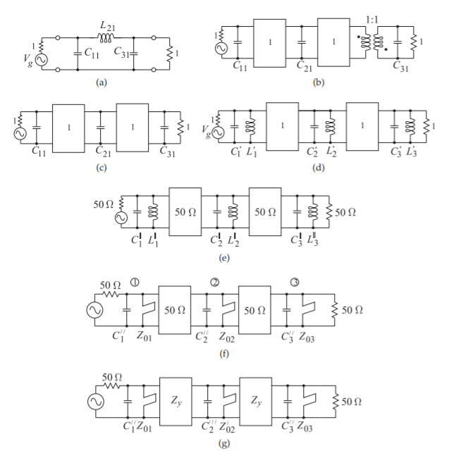
Figure \(\PageIndex{1}\): Early prototypes in the development of a third-order Butterworth combline filter.

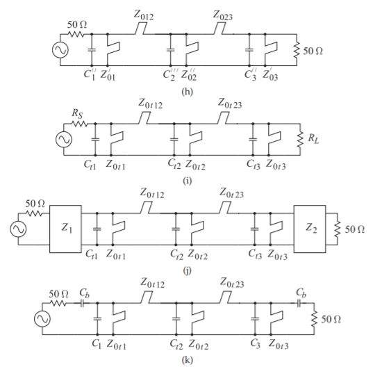
Figure \(\PageIndex{2}\): Late-stage prototypes in the development of a third-order Butterworth combline filter.