4.5: Oscillator Noise

Noise on oscillators has a particular characteristic that affects the use of oscillators in RF systems. When oscillating, the frequency of oscillation varies slightly and this variation is captured as phase noise.

4.4.1 Observations of Noise Spectra of Oscillators

In the frequency domain, noise is characterized by its power spectral density, \(S\), which is the noise power in a specified bandwidth. It is typical to use \(1\text{ Hz}\) as the reference bandwidth and then \(S\) is expressed in units of watts per hertz or, more commonly, as \(\text{dBm}\) per hertz. Some types of noise are proportional to the RF signal or carrier level and are expressed relative to the level of the carrier as \(\text{dBc/Hz}\) (\(10 \log\) of the ratio of the noise power per hertz relative to the power of the carrier). Noise can be decomposed into a phase component, \(S_{\varphi}\), and an amplitude component, \(S_{a}\). Then the observed phase fluctuations, as classified in [18], are as shown in Figure \(\PageIndex{1}\). There are also amplitude fluctuations that have a similar characteristic. For example, flicker amplitude noise will also have an \(f^{−1}\) dependence. However, the phase component generated by electronic circuits gets the most attention as small amplitude variations are quenched by device nonlinearities. In Figure \(\PageIndex{1}\), the log of

Frequency \((\text{GHZ})\)	\(F_{\text{min}}\)	\(\text{NF}_{\text{min}}\) \((\text{dB})\)	\(\Gamma_{n}\)	\(\angle\Gamma_{n}\) degrees	\(r_{n}/50\) \((\Omega )\)
\(0.90\)	\(1.07\)	\(0.29\)	\(0.747\)	\(15.70\)	\(0.165\)
\(1.80\)	\(1.09\)	\(0.38\)	\(0.623\)	\(24.95\)	\(0.176\)
\(2.40\)	\(1.11\)	\(0.44\)	\(0.795\)	\(37.45\)	\(0.158\)
\(2.60\)	\(1.11\)	\(0.47\)	\(0.640\)	\(47.15\)	\(0.159\)
\(2.80\)	\(1.12\)	\(0.49\)	\(0.670\)	\(47.90\)	\(0.160\)
\(3.20\)	\(1.13\)	\(0.53\)	\(0.617\)	\(51.20\)	\(0.156\)
\(4.00\)	\(1.15\)	\(0.61\)	\(0.542\)	\(68.70\)	\(0.141\)
\(5.00\)	\(1.18\)	\(0.72\)	\(0.465\)	\(85.00\)	\(0.120\)
\(5.50\)	\(1.19\)	\(0.77\)	\(0.431\)	\(91.10\)	\(0.114\)
\(6.00\)	\(1.21\)	\(0.83\)	\(0.366\)	\(101.15\)	\(0.107\)
\(7.00\)	\(1.24\)	\(0.93\)	\(0.262\)	\(122.10\)	\(0.096\)
\(8.00\)	\(1.27\)	\(1.04\)	\(0.188\)	\(153.60\)	\(0.100\)
\(9.00\)	\(1.30\)	\(1.14\)	\(0.135\)	\(-165.60\)	\(0.121\)
\(10.00\)	\(1.33\)	\(1.25\)	\(0.162\)	\(-126.80\)	\(0.138\)
\(11.00\)	\(1.37\)	\(1.35\)	\(0.183\)	\(-85.95\)	\(0.187\)
\(12.00\)	\(1.40\)	\(1.46\)	\(0.270\)	\(-68.40\)	\(0.239\)
\(13.00\)	\(1.43\)	\(1.57\)	\(0.343\)	\(-50.25\)	\(0.355\)
\(14.00\)	\(1.47\)	\(1.67\)	\(0.431\)	\(-43.95\)	\(0.461\)
\(15.00\)	\(1.51\)	\(1.78\)	\(0.573\)	\(-25.80\)	\(0.604\)

Table \(\PageIndex{1}\): Noise parameters of an enhancement-mode pHEMT transistor model FPD6836P70 [17]. \(F_{\text{min}}\) is the minimum noise factor, \(\text{NF}_{\text{min}}\) is the minimum noise figure, and \(\Gamma_{n} = \Gamma_{\text{opt}}\) is the source reflection coefficient yielding \(F_{\text{min}}\).

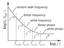
Figure \(\PageIndex{1}\): Wideband noise showing only phase and frequency noise. \(S_{\varphi}\) is the spectral density of the phase noise and \(f\) is frequency.

the phase noise power spectral density relative to a reference level is plotted as a function of the log of frequency. The graph does not go all the way down to DC because the frequency axis is logarithmic. This does not imply that the noise power goes to infinity\(^{1}\) as, of course, the bandwidth is becoming smaller and smaller at low \(\log(f)\).

Figure \(\PageIndex{1}\) is the usual way to plot noise, as straight-line regions are clearly observed experimentally and in these regions the noise power spectral density varies with frequency as \(1/f^{n}\), where \(n\) is a positive integer. Sometimes one or more of these regions will be missing, and this is interpreted as the crossover frequencies, the \(f_{c−n}\)s in Figure \(\PageIndex{1}\), being out of order.

The observed noise characteristic (Figure \(\PageIndex{1}\)) is intriguing. Why are there straight line regions and what are the physical processes that produce noise with such characteristics? The straight-line regions are in contrast to what could, perhaps, be expected to be a smooth continuous transition from a low spectral density region to a high spectral density region.

Names have been given to the regions [18], with the first being white phase noise, noise with no frequency dependence (i.e., a frequency dependence of \(f^{0}\)). This noise has a mean and a variance but no higher (i.e., third and above) moment. In the time domain this noise has (actually assumed to have) a Gaussian distribution. This is the form of noise that can be translated between the time and frequency domains using integer calculus.

The next noise region seen in Figure \(\PageIndex{1}\) is called the flicker phase noise region with noise spectral density dependent on \(1/f\) (or \(f^{−1}\)). Traditionally this has been a puzzling noise characteristic and is possibly due to chaotic behavior. The \(1/f\) characteristic indicates that there is long-term memory, which is the same as saying that fluctuations (i.e., noise) are correlated to fluctuations at past times. In RF and microwave systems, flicker phase noise is often the most significant noise and sets the noise-related performance limits receiver circuits in particular. Energy consumption is also affected as flicker noise is usually suppressed by increasing oscillator bias currents. Following the \(1/f\) region are the white frequency, \(f^{−2}\), flicker frequency, \(f^{−3}\), and random walk frequency regions, \(f^{−4}\). These regions also indicate longterm correlation of fluctuations. It has been shown that at least some of the noise in the \(f^{−2}\) region is die to up-converted white noise from near DC [22] and from white noise near harmonics of the oscillating signal [23].

At RF the noise of greatest interest is the noise superimposed on a signal that is amplified, or the noise that is generated by an oscillator. This noise has a white noise component and one or more components with \(1/(\Delta f)^{n}\) dependence, where \(n\) is a positive integer and \(\Delta f\) is the offset from the center signal frequency. The noise with \(1/(\Delta f)^{n}\) dependence has been found to

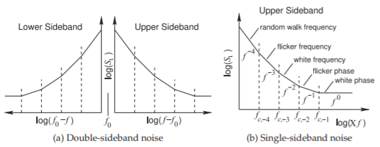
Figure \(\PageIndex{2}\): Narrowband noise around the carrier frequency, \(f_{0}\), of an oscillator showing only phase and frequency noise with \(\Delta f = f − f_{0}\).

be at least partly related to the noise observed at low frequencies. (This is another indication of our lack of a full understanding of noise.)

The phase noise observed on the signal produced by an oscillator is shown in Figure \(\PageIndex{2}\)(a). While the noise appears both above and below the oscillating frequency, so-called double-sideband noise, usually only the upper sideband is plotted, as shown in Figure \(\PageIndex{2}\)(b). The designations of the straight-line regions [18] (see Figure \(\PageIndex{2}\)(b)) correspond to the designations for low-frequency noise (see Figure \(\PageIndex{1}\)). The noise observed on an oscillation signal or on the signal at the output of an amplifier must, necessarily, come from processing of a physical noise source.

The noise on the signal at the output of an oscillator is almost entirely phase fluctuations, as saturation quenches amplitude fluctuations. Phase fluctuations in the frequency domain are characterized by spectral density of the phase fluctuations. If the signal at the output of the oscillator is

\[\label{eq:1}v(t)=[V_{0}+\epsilon (t)]\sin[2\pi f_{0}t+\phi(t)] \]

where \(\epsilon (t)\) is the amplitude fluctuation and \(\phi (t)\) is the phase fluctuation, the spectral density of phase fluctuations is

\[\label{eq:2}S_{\phi}(\Delta f)=S_{\phi}(\Delta\omega)=\text{PSD}[\phi (t)]=\frac{E[\phi^{2}(t)]}{B} \]

where \(\Delta f = \Delta\omega /(2\pi )\) is the frequency offset from the carrier at frequency \(f_{0}\), \(\text{PSD}\) refers to power spectral density, \(E[\:]\) refers to the estimated value (here the mean of the squared phase), and \(B\) is the bandwidth over which the estimate is made (i.e., the bandwidth of the measurement). With bandwidth having the units of hertz, then the units of \(S_{\phi}\) are radians\(^{2}/\text{Hz}\). Equation \(\eqref{eq:2}\) includes contributions from both the upper and lower sidebands and so it is a double-sideband measure of phase noise. The preferred measure is the single-sideband phase noise spectral density \(\mathcal{L}\) (read as script-L) so that\(^{2}\)

\[\label{eq:3}\mathcal{L}(f)=\frac{1}{2}S_{\phi}(f) \]

Footnotes

[1] More importantly, the integration, using integer calculus, is not valid. The noise that has the \(1/f\)-like spectrum is believed to be fractal (i.e., of chaotic origin). Fractals are formally irregular, rough, and nondifferentiable. That is, fractal processes are inaccessible to treatment by integer calculus and thus they do not have a power spectrum [19]. However, it has been shown that such a process when passed through an ideal bandpass filter will become stationary and then have a power spectrum [20, 21]. What this means is that since measurement equipment is band limited, the measured spectrum may appear to approach infinity as the offset goes to zero, but the underlying physical noise process will not. As well, the real bandpass filter of measurement equipment has loss and so a measurement artifact is that noise measurements will level off for smaller and smaller frequency offsets.

[2] In the past, \(\mathcal{L}(f)\) was defined as the single-sideband noise power in a \(1\text{ Hz}\) bandwidth divided by the carrier power. This definition has been superseded by Equation \(\eqref{eq:3}\) because of ambiguities in applying the old definition when both amplitude and phase fluctuations are significant.