4.6: Nonlinear Distortion

Distortion imposes a fundamental limit to the efficiency that can be realized in an RF system [24, 25, 26, 27]. There must be enough DC power to ensure that signals are processed with no more than the maximum acceptable distortion. Nonlinear distortion originates when the output signal from an amplifier, for example, approaches the extremes of the load line so that the output is not an exact amplified replication of the input signal.

4.5.1 Amplitude and Phase Distortion

For a one-tone signal, the amplitude gain of the signal rolls off as the input power increases, as shown in Figure \(\PageIndex{1}\)(a). This figure plots the power of the output sinewave against the power of the input sinewave. The plot is called the AM-to-AM (AM-AM) response (the amplitude-dependent amplitude response) of the amplifier. The AM-AM characteristic is linear at low input powers, but eventually the gain reduces (compresses) and the output power drops below the linear extension of the small-signal response. In Figure \(\PageIndex{1}\)(a), the \(1\text{ dB}\) gain compression point is the point where the difference between the extrapolated linear response exceeds the actual gain by \(1\text{ dB}\). \(P_{1\text{dB}}\) is the output power at the \(1\text{ dB}\) gain compression point and is the single most important metric of distortion, and amplifier designers use \(P_{1\text{dB}}\) as a point of reference.

A gain compression of \(1\text{ dB}\) corresponds to a signal voltage amplitude reduction of \(11\%\) so \(P_{1\text{dB}}\) indicates a small but significant reduction in the linear gain of an amplifier. For high orders of modulation this \(11\%\) error could mean that the sampled received signal does not match the actual transmitted constellation point. The range of power of a modulated input signal is usually chosen so that the peak power of the envelope is equal to or less than the \(1\text{ dB}\) gain compression power. Thus for nearly all modulation formats (a notable exception is FM) the average signal power is backed-off from the \(1\text{ dB}\) gain compression power by the peak-to-mean envelope power ratio (PMEPR) of the modulated signal. With higher-order modulation having a higher PMEPR a greater back-off is required.

At large powers, the parasitic capacitances of the transistors in the amplifier vary the phase of the output signal, and hence phase distortion occurs. Figure \(\PageIndex{1}\)(b) shows what is called the AM-to-PM (AM-PM) characteristic which is a measure of the amplitude-dependent phase distortion. For a digitally modulated signal, phase distortion would be

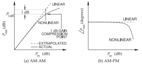
Figure \(\PageIndex{1}\): Nonlinear effects introduced by RF hardware: (a) amplitude-dependent amplitude (AM-AM) distortion; and (b) amplitude-dependent phase (AM-PM) distortion.

significant if it caused the wrong constellation point to be selected in a receiver. So for 8-PSK modulation a \(22.5^{\circ}\) phase shift would be significant, less if noise is considered. The AM-AM distortion generally occurs before the output phase varies appreciably. This is because the nonlinearity of a transistor is predominantly a current-voltage nonlinearity with phase distortion coming mostly from the nonlinearity of parasitic capacitances.

While Figure \(\PageIndex{1}\) presents the distortion characteristics for a single sinewave, it has proved to be a reasonable indicator of performance with modulated signals. In particular, with the maximum peak envelope output power being \(P_{1\text{dB}}\), in-band distortion is usually acceptable while maximizing high amplifier efficiency [28].

The AM-AM and AM-PM characterizations describe distortion with an amplifier but they are also used with other types of nonlinear subsystems such as mixers.

Example \(\PageIndex{1}\): Amplifer Back-Off

An amplifier has an output power of \(10\text{ dBm}\) when the gain of a single tone is compressed by \(1\text{ dB}\). What is the maximum output power of an undistorted QPSK signal with a PMEPR of \(3.6\text{ dB}\)?

Solution

The maximum undistorted output QPSK signal is generally accepted as being when the peak envelope power is equal to the \(1\text{ dB}\) gain compression power. In dBm the peak envelope power is greater than the mean signal power by the peak-to-mean envelope power ratio. Thus the QPSK signal power is said to be backed-off from the \(1\text{ dB}\) gain compression point by PMEPR. Thus the maximum undistorted output power of the QPSK signal is

\[\label{eq:1}P_{o,\text{QPSK}}=P_{1\text{dB}}|_{\text{dBm}}-\text{PMEPR}|_{\text{dB}}=10\text{ dBm}-3.6\text{ dB}=6.4\text{ dBm} \]

4.5.2 Gain Compression

The voltage \(v_{o}(t)\) at the output of an amplifier that is biased in the middle of the output current-voltage characteristics (i.e., a Class A amplifier) can be modeled by the first few terms of a Taylor series

\[\label{eq:2}v_{o}(t)=a_{0}+a_{1}v_{i}(t)+a_{2}v_{i}^{2}(t)+a_{3}v_{i}^{3}(t)+\ldots \]

where \(v_{i}(t)\) is the input voltage. In a Class A amplifier, the even-order terms are small because distortion at the extremes of the voltage waveform are largely symmetrical, and it is found that the coefficients of the odd-order terms of the Taylor series rapidly decrease so that \(|a_{1}|≫|a_{3}|≫|a_{5}|\ldots\). Also it is found that \(a_{3}\) is negative. With a single sinusoidal input voltage at frequency \(f_{1} = \omega_{1}/(2\pi)\), \(v_{i}(t) = V_{1} \cos(\omega_{1}t)\) and the output voltage is

\[\begin{align}v_{o}(t)&=a_{0}+a_{1}V_{i}\cos(\omega_{1}t)+a_{2}V_{1}^{2}\cos^{2}(\omega_{1}t)+a_{3}V_{i}^{3}\cos^{3}(\omega_{1}t)+\ldots\nonumber \\ &=(a_{0}+\frac{1}{2}a_{2}V_{i}^{2})+(a_{1}V_{i}+\frac{3}{4}a_{3}V_{i}^{3})\cos(\omega_{1}t)\nonumber \\ \label{eq:3}&\quad+\frac{1}{2}a_{2}V_{i}^{2}\cos(2\omega_{1}t)+\frac{1}{4}a_{3}V_{i}^{3}\cos(3\omega_{1}t)+\ldots\end{align} \]

RF and microwave amplifiers are used with bandpass filters and the distortion corresponding to harmonics is easily filtered out. Thus the output, after filtering and removing the DC component is

\[\label{eq:4}v_{o}(t)=(a_{1}V_{i}+\frac{3}{4}a_{3}V_{i}^{3})\cos(\omega_{1}t)=V_{o}\cos(\omega_{1}t) \]

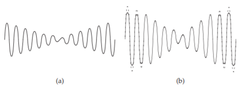
Figure \(\PageIndex{2}\): A twotone signal: (a) a two-tone input waveform; and (b) distorted output showing compression (dashed waveform is undistorted).

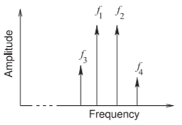
Figure \(\PageIndex{3}\): Spectrum at the output of a nonlinear amplifier with a two-tone input signal. This is the spectrum of the waveform in Figure \(\PageIndex{2}\). Numerically \(f_{3} = 2f_{1} − f_{2}\) and \(f_{4} = 2f_{2} − f_{1}\).

where \(V_{o} = a_{1}V_{i} + \frac{3}{4}a_{3}V_{i}^{3}\) is the magnitude of the voltage at the input frequency. So the voltage gain is

\[\label{eq:5}^{V}G=\frac{V_{o}}{V_{i}}=a_{1}+\frac{3}{4}a_{3}V_{i}^{2} \]

and the power gain (assuming the input and output impedances are the same) is

\[\label{eq:6}G=\:^{V}G^{2} \]

Since \(a^{3}\) is negative, the gain for very low input voltages, small \(V_{1}\), is linear with \(^{V}G = a_{1}\) and the gain reduces for larger input signals, resulting in the gain compression, the reduction in the slope of \(P_{\text{out}}\) versus \(P_{\text{in}}\), seen in Figure \(\PageIndex{1}\)(a). For other amplifiers, and particularly for switching amplifiers, many more terms must be considered in the power series expansion, and it is possible that the gain could increase before dropping and eventually saturating. This temporary increase in gain is called gain expansion.

4.5.3 Intermodulation Distortion

A two-tone signal consisting of two sinusoidal signals is a better representation of system performance with modulated signals. A signal that is the linear combination of two sinusoidal signals of equal amplitude is shown in Figure \(\PageIndex{2}\)(a). When this signal is large and is input to an amplifier in what is called a two-tone test, the extremes of the output signal are compressed. This results in the saturated output waveform shown in Figure \(\PageIndex{2}\)(b), where the dashed curve is the undistorted waveform. In the frequency domain this distortion produces additional tones so that this distortion is said to produce intermodulation products (IMPs), as shown in Figure \(\PageIndex{1}\). Here the \(f_{1}\) and \(f_{2}\) components have the frequencies of the original two-tone input signal. The extra tones in the output, \(f_{3}\) and \(f_{4}\), are the intermodulation tones. The tone at \(f_{3} = 2f_{1} − f_{2}\) is known as the lower IM3 (or lower third-order intermod) tone and the tone at \(f_{4} = 2f_{2} − f_{1}\) is known as the upper IM3 tone.

The simplest way to view intermodulation distortion is to consider a twotone input signal,

\[\label{eq:7}v_{i}(t)=V_{i}[\cos(\omega_{1}t)+\cos(\omega_{2}t)] \]

where the tones at frequencies \(f_{1} = \omega_{1}/(2\pi )\) and \(f_{2} = \omega_{2}/(2\pi)\) have equal amplitude \(V_{i}\). Substituting this signal into the Taylor series expansion in Equation \(\eqref{eq:2}\) leads to the output signal

\[\begin{align}v_{o}(t)&=a_{0}+a_{1}V_{i}\cos(\omega_{1}t)+a_{1}V_{i}\cos(\omega_{2}t)+\frac{1}{2}a_{2}V_{i}^{2}[\cos(\omega_{1}t)+\cos(\omega_{2}t)]^{2}\nonumber \\ &\quad +a_{3}V_{i}^{3}[\cos(\omega_{1}t)+\cos(\omega_{2}t)]^{3}+\ldots\nonumber \\ &=a_{0}+a_{1}V_{i}\cos(\omega_{1}t)+a_{1}V_{i}\cos(\omega_{2}t)+\frac{1}{2}a_{2}V_{i}^{2}[1+\cos(2\omega_{1}t)]\nonumber \\ &\quad +\frac{1}{2}a_{2}V_{i}^{2}[1+a_{1}\cos(2\omega_{2}t)]+a_{2}V_{i}^{2}\cos(\omega_{1}-\omega_{2})t+a_{2}V_{i}^{2}\cos(\omega_{1}+\omega_{2})t\nonumber \\ &\quad +a_{3}V_{i}^{3}[\frac{3}{4}\cos(\omega_{1}t)+\frac{1}{4}\cos(3\omega_{1}t)]+a_{3}V_{i}^{3}(\frac{3}{4}\cos(\omega_{2}t)+\frac{1}{4}\cos(3\omega_{2}t)]\nonumber \\ &\quad +a_{3}V_{i}^{3}[\frac{3}{2}\cos(3\omega_{1}t)+\frac{3}{4}\cos(2\omega_{2}-\omega_{1})t+\frac{3}{4}\cos(2\omega_{2}+\omega_{1})t]\nonumber \\ \label{eq:8}&\quad+ a_{3}V_{i}^{3}[\frac{3}{2}\cos(3\omega_{2}t)+\frac{3}{4}\cos(2\omega_{1}-\omega_{2})t+\frac{3}{4}\cos(2\omega_{1}+\omega_{2})t]+\ldots\end{align} \]

The component of the output at the first fundamental is

\[\label{eq:9}V_{o,1}=a_{1}V_{i}+\frac{3}{4}a_{3}V_{i}^{3} \]

and the component of the output at the second fundamental is

\[\label{eq:10}V_{o,2}=a_{1}V_{i}+\frac{3}{4}a_{3}V_{i}^{3} \]

Note that \(a_{1}\) is the linear voltage gain of the amplifier:

\[\label{eq:11}a_{1}=V_{o,1}/V_{i}=V_{o,2}/V_{i} \]

4.5.4 Third-Order Distortion

RF and microwave amplifiers are typically used with bandpass or lowpass inter-stage matching networks or filters, and so the distortion corresponding to harmonics is filtered out. However, the tones at frequency \(f_{3} = 2f_{1} − f_{2} = \omega_{3}/(2\pi)\) and \(f_{4} = 2f_{1} − f_{2} = \omega_{4}/(2\pi )\) will be within the passband of the amplifier if f1 and f2 are close. The appearance of these tones indicates third-order distortion as the distortion is the result of third-order terms in the power series expansion of the two-tone input-output characteristic as given in Equation \(\eqref{eq:8}\). That is, the output after filtering and removing the DC component is

\[\label{eq:12}v_{o}(t)=V_{0,1}\cos(\omega_{1}t)+V_{o,2}\cos(\omega_{2}t)+V_{o,3}\cos(\omega_{3}t)+V_{o,4}\cos(\omega_{4}t) \]

where the component of the output

\[\begin{align}\label{eq:13}\text{at the first fundamental, }f_{1},\text{ is }V_{o,1}&=a_{1}V_{i}+\frac{3}{4}a_{3}V_{i}^{3}\\ \label{eq:14}\text{at the second fundamental, }f_{2},\text{ is }V_{o,2}&=a_{1}V_{i}+\frac{3}{4}a_{3}V_{i}^{3} \\ \label{eq:15}\text{at the lower intermodulation frequency, }f_{3},\text{ is }V_{o,3}&=\frac{3}{4}a_{3}V_{i}^{3} \\ \label{eq:16}\text{at the upper intermodulation frequency, }f_{4},\text{ is }V_{o,4}&=\frac{3}{4}a_{3}V_{i}^{3}\end{align} \]

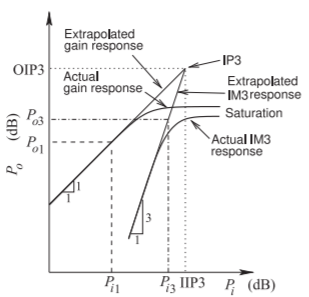
Figure \(\PageIndex{4}\): Output power versus input power of an amplifier plotted on a logarithmic scale. The IM3 response is a result of two-tone intermodulation, and the input power is the power of each of the two signals that have equal amplitude. Extrapolations of the \(1:1\) linear fundamental response and the \(3:1\) third-order intermodulation response intersect at the IP3 point.

Thus the level of the intermodulation tones, the IMD level, increases as the third power of the level of the two-tone input signal. Since the IMD levels vary as the third power of the input tone level (\(V_{i}\)), it is usual to refer to the tones at \(f_{3}\) and \(f_{4}\) as third-order intermods, or IM3 tones. The one-tone and IM3 responses are plotted in Figure \(\PageIndex{4}\) up until saturation, where higher-order terms in the Taylor expansion become important.

The ratio of the amplitude of the intermodulation tones to the amplitude of the input tones (recall that they have equal amplitude) enables the thirdorder power series coefficient to be calculated. That is

\[\label{eq:17}a_{3}=\frac{4}{3}\frac{V_{o,3}}{V_{i}^{3}}=\frac{4}{3}\frac{V_{o,4}}{V_{i}} \]

The gain and IM3 responses shown in Figure \(\PageIndex{4}\) are plotted on a logarithmic scale. First consider the gain response, which is plotted for a single sinewave input. At low input power levels the amplifier has linear gain and the output power, \(P_{o1}\), increases in proportion to the input power, \(P_{i1}\), so the gain response has a \(1:1\) slope. As the input power further increases, the output power saturates primarily because the waveform at the output is constrained by the limits set by the supply and ground rails, but other nonlinearities of the transistor impact the linearity of the response before saturation is reached. The IM3 response (either the level of the \(f_{3}\) tone or the \(f_{4}\) tone) in Figure \(\PageIndex{4}\) is when the levels of two discrete tones are the same. Then typically the responses of the upper and lower IM3 tones are the same unless capacitive effects become important [29, 30, 31, 32]. At low levels of the two input tones, each with power \(P_{i3}\), the output power, \(P_{o3}\), at one of the IM3 tones increases as the third power of \(P_{i3}\). Thus on a logarithmic scale the slope of \(P_{o3}\) versus \(P_{i3}\) is \(3:1\). As the input power increases the IP3 response eventually saturates. The two simplest characterizations of the nonlinear response of an amplifier are the \(1\text{ dB}\) gain compression power, as discussed before, and the intercept of the gain and IP3 responses. This intersection is called the third-order intercept point, or IP3 point (see Figure \(\PageIndex{4}\)). The input power at IP3 is called the input third-order intercept power, or IIP3, and the output is called the output third-order intercept power, or OIP3. If \(G\) is the linear power gain, \(\text{OIP3} = G\cdot \text{IIP3}\). IIIP3 is mostly used with receivers and OIP3 is used with transmitters.

4.5.5 Spectral Regrowth

Distortion with digitally modulated signals consists of in-band and out-of-band distortion. The generation of in-band (within the bandwidth of the digitally modulated signal) intermodulation distortion in an amplifier, or any other nonlinear device such as a mixer, affects the ability to resolve the constellation of a received signal. Thus distortion generated in-band affects the ability to interpret the constellation of the signal and hence causes bit errors. However, the phase of the intermodulation products is of little concern except in cascaded systems where the phase affects how IMD distortion from different stages combines.

Out-of-band distortion is represented in Figure \(\PageIndex{5}\), where the spectra at the input and output of a nonlinear system are shown. The process that results in increased signal levels in the adjacent sidebands is called spectral regrowth. This distortion is similar to the intermodulation distortion with a two-tone signal. The generation of signals in the adjacent channel affects the function of other radios and the allowable level of these signals is contained in system specifications.

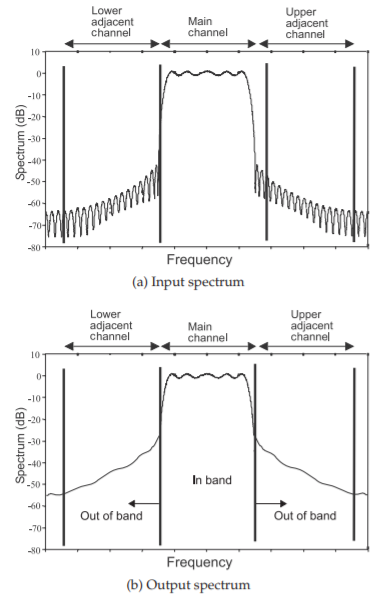
Figure \(\PageIndex{5}\): Spectra at the input and output of an amplifier with of a digitally modulated signal.

4.5.6 Second-Order Distortion

The previous subsection discussed intermodulation distortion and introduced the third-order intercept point, IP3, defined either by the input-referred power of IP3, IIP3, or the output-referred power of IP3, OIP3, to characterize third-order nonlinear performance. The same type of analysis can be used to characterize the second-order nonlinear performance of a microwave module. Second-order distortion leads to the second harmonic of the input tones and to the difference frequency of the input tones. The components of the output response of the amplifier in Equation \(\eqref{eq:8}\) at the second harmonic and difference frequency are:

\[\label{eq:18}v_{0}(t)=V_{0,2\text{nd},1}\cos(2\omega_{1}t)+V_{0,2\text{nd},2}\cos(2\omega_{2}t)+V_{o,\text{diff}}\cos(\omega_{2}-\omega_{1}t) \]

where the amplitude at the output at the

\[\begin{align}\text{second harmonic of }f_{1}\text{ is }V_{0,2\text{nd},1}&=\frac{1}{2}a_{2}V_{i}^{2}\nonumber \\ \text{second harmonic of }f_{2}\text{ is }V_{0,2\text{nd},2}&=\frac{1}{2}a_{2}V_{i}^{2}\nonumber \\ \label{eq:19}\text{difference frequency }f_{2}-f_{1}\text{ is }V_{0,\text{diff}}&=\frac{1}{2}a_{2}V_{i}^{2}\end{align} \]

Thus the coefficient of the second-order term in the defining polynomial can be obtained from the amplitude of either of the second harmonics or of the difference tone.

\[\label{eq:20}a_{2}=2\frac{V_{0,2\text{nd},1}}{V_{i}^{2}}=2\frac{V_{0,2\text{nd},2}}{V_{i}^{2}}=2\frac{V_{0,\text{niff}}}{V_{i}^{2}} \]

The gain and IM2 responses shown in Figure 4.6.1 are plotted on a logarithmic scale. At low input power levels the amplifier has a linear gain and initially the gain response has a \(1:1\) slope. The IM2 response (either the levels of the second harmonic tones or of the difference tone) in Figure 4.6.1 is when the levels of two discrete tones are the same. At low levels of the two input tones, each with power \(P_{i2}\), the output power, \(P_{o2}\), at one of the harmonic or difference tones increases as the quadratic of \(P_{i32}\). Thus on a logarithmic scale the slope of \(P_{o2}\) versus \(P_{i2}\) is \(2:1\). As the input power increases the IP2 response eventually saturates. The simplest characterizations of the second-order nonlinear response of an amplifier is the IP2 response and the IP2 intercept point, the second-order intercept point. The input power at IP2 is called the input second-order intercept power, or IIP2, and the output is called the output second-order intercept power, or OIP2.

4.5.7 Summary

The three simplest characterizations of the performance of an amplifier are the linear gain, the input or output power at the IM2 intercept point, IP2, and the input or output power at the IM3 intercept point, IP3, see Figures 4.6.1 and 4.6.2. From these the first three coefficients of a polynomial model of an amplifier can be derived. The first, \(a_{1}\), comes from the linear gain, see. The second, \(a_{2}\), comes from the level of the harmonics or difference tones for a two-tone input signal, see Equation \(\eqref{eq:20}\). The third, \(a_{3}\) comes from the level of third-order intermodulation tones, see Equation \(\eqref{eq:17}\).