7.2: Nonlinear Distortion of a Cascaded System

This section builds on the distortion analysis of two-port networks in Section 4.5 and addresses the determination of the nonlinear metrics of a cascaded system such the receiver shown in Figure 7.1.2. The filters and interstage matching networks eliminate harmonics from the system but, unfortunately, allow in-band and close-in out-of-band distortion components to pass through the system. The main metrics that describe nonlinear performance are the power levels at the \(1\text{ dB}\) gain compression point and at the third-order intercept (\(\text{IP3}\)) point. In some systems, such as direct-conversion receivers, the second-order intercept point (\(\text{IP2}\)) is also important. These metrics relate to discrete tones and the correlated distortion generated in the different stages. This contrasts with the calculation of noise of a cascaded system where the noise added by stages is uncorrelated.

Gain Compression in a Cascaded System

When two amplifier stages are cascaded it is necessary to determine the \(1\text{ dB}\) gain compression point of the cascade. Consider the cascade in Figure \(\PageIndex{1}\). The two stages have linear power gains \(G_{1}\) and \(G_{2}\), and \(1\text{ dB}\) compression points \(P_{1, 1\text{ dB}}\) and \(P_{2,1 \text{dB}}\), respectively. The total linear power gain of the system is \(G^{T} = G_{1}\cdot G_{2}\). If the Taylor series expansion of the input-output characteristics of the first stage in the cascade is

\[\label{eq:1}v_{1o}(t)=a_{0}+a_{1}v_{1i}(t)+a_{2}v_{1i}^{2}(t)+a_{3}v_{1i}^{3}(t)+\ldots \]

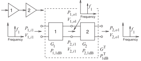
Figure \(\PageIndex{1}\): Cascade of two stages used in determining the total \(1\text{ dB}\) compression point of the system.

then at the interface of the two stages the amplitude of the tone at \(f_{1}\) due to a single-tone input, \(v_{i}(t) = V_{i} \cos(\omega_{1}t)\), is \(v_{1o}(t) = V_{1o} \cos(\omega_{1}t)\), where

\[\label{eq:2}V_{1o}=a_{1}V_{i}+\frac{3}{4}a_{3}V_{i}^{3} \]

The harmonics are ignored, as design of the interstage matching network would preferably be lowpass to eliminate the passage of harmonics. The input of the second stage is \(v_{2i}(t) = v_{1o}(t)\), with the Taylor series expansion of the second stage being

\[\label{eq:3}v_{2o}(t)=b_{o}+b_{1}v_{2i}(t)+b_{2}v_{2i}^{2}(t)+b_{3}v_{1i}^{3}(t)+\ldots \]

Thus the component of the final output at \(f_{1}\) will be

\[\label{eq:4}V_{o}=a_{1}b_{1}V_{i}+\frac{3}{4}b_{1}a_{3}V_{i}^{3}+\frac{3}{4}a_{1}b_{3}V_{i}^{3}+\ldots \]

That is, the input signal is multiplied by the overall linear gain of the amplifier; this is the first term on the right in Equation \(\eqref{eq:4}\), and the last two terms result in gain compression. If the stages are identical (i.e., \(a_{1} = b_{1}\) and \(a_{3} = b_{3}\)) the two gain compression terms will be identical. Thus the two stages will contribute equally to gain compression.

Note that in Equation \(\eqref{eq:4}\) voltages add to yield the overall gain compression. In general the two stages will not be identical, they will have different gain and \(1\text{ dB}\) compression points, however, this observation (i.e., that the voltages add) does enable an approximate expression to be developed for the \(1\text{ dB}\) compression point of a cascaded system.

Examination of Equation \(\eqref{eq:4}\) leads to a general formula for the total \(1\text{ dB}\) compression point, \(P_{1\text{dB}}^{T}\), of the two-stage cascade in Figure \(\PageIndex{1}\):

\[\label{eq:5}(P_{1\text{dB}}^{T})^{-\frac{1}{2}}\approx (G_{2}P_{1,1\text{ dB}})^{-\frac{1}{2}}+(P_{2,1\text{ dB}})^{-\frac{1}{2}} \]

Note that here the gains and the powers are absolute quantities and not in decibels. For example, \(P_{1\text{dB}}^{T}\) is the power in watts at the \(1\text{ dB}\) gain compression point.

Equation \(\eqref{eq:5}\) is a very conservative estimate of the \(1\text{ dB}\) gain compression point of the amplifier and flags the lowest power levels at which gain compression of the cascade could occur. The situation could be better depending on the phasing of the distortion components but conservatism is very important in system design. The worst case is what matters in specifying system performance. Getting the effect of phasing right in system design requires a circuit-level simulation but when working with modules such information is rarely available. Equation \(\eqref{eq:5}\) cannot be directly derived from the voltage expansion as the power gain of microwave amplifiers is due to difference of input and output impedance levels in addition to voltage gain. It should be noted that a microwave amplifier deviates from linearity following a sharper, tanh-like, response than that described by a low-order polynomial model of linearity. Thus simply cascading low-order polynomials describing each stage is not a viable option.

If required and if a more realistic estimate is required and can be justified, then a less conservative formula that can be used to estimate the gain compression level of two cascaded stages is

\[\label{eq:6}(P_{1\text{ dB}}^{T})^{-1}\approx (G_{2}P_{1,1\text{ dB}})^{-1}+(P_{2,1\text{ dB}})^{-1} \]

It is usually better to use the more conservative estimate of compression in Equation \(\eqref{eq:5}\).

Example \(\PageIndex{1}\): Gain Compression of a Two-Stage Amplifier

The first stage of a two-stage amplifier in a transmitter has a gain \(G_{1} = 20\text{ dB}\) and an output \(1\text{ dB}\) gain compression power \(P_{1,1\text{ dB}} = 10\text{ dBm}\). The second stage has a gain \(G_{2} = 6\text{ dB}\) and an output \(1\text{ dB}\) gain compression power \(P_{2,1\text{ dB}} = 20\text{ dBm}\).

1. What is the linear gain of the two-stage amplifier?
2. What is the gain of the two-stage amplifier at the \(1\text{ dB}\) gain compression power?
3. What is the \(1\text{ dB}\) gain compression power of the cascaded system?

Solution

1. When the gain of an amplifier stage is given without qualification it should be assumed to be the linear gain, that is, the gain at small signal levels. So the total linear power gain of the two-stage amplifier is
   \[G^{T}=G_{1}G_{2}=20\text{ dB}+6\text{ dB}=26\text{ dB}\nonumber \]
2. The compressed gain will be \(1\text{ dB}\) less, that is, \(G^{T} = 25\text{ dB}\).
3. The overall gain compression power, \(P^{T}_{1\text{ dB}}\) is, approximately obtained using Equation \(\eqref{eq:5}\):
   \[\begin{align}\left(P_{1\text{ dB}}^{T}\right)^{-\frac{1}{2}}&=(G_{2}P_{1,1\text{ dB}})^{-\frac{1}{2}}+(P_{2,1\text{ dB}})^{-\frac{1}{2}} = \left(10^{(6/10)}10^{(10/10)}\right)^{-\frac{1}{2}}+\left(10^{(20/10)}\right)^{-\frac{1}{2}}\nonumber\\ \label{eq:7}P_{1\text{ dB}}^{T}&=\left[(3.981\cdot 10)^{-\frac{1}{2}}+(100)^{-\frac{1}{2}}\right]^{-2}\text{ mW}=14.97\text{ mW}=11.8\text{ dBm}\end{align} \]
   A quick check is as follows.
   If Stage \(1\) dominates gain compression, the output power at the \(1\text{ dB}\) compression is \(P_{1,1\text{ dB}} = 10\text{ dBm}\) multiplied by the linear power gain of the second stage, that is, \(P^{T}_{1\text{ dB}} = G_{2}P_{1,1\text{ dB}} = 6\text{ dB} + 10\text{ dBm} = 16\text{ dBm}\).
   If Stage \(2\) dominates compression, the output power at the \(1\text{ dB}\) compression of the two-stage amplifier is just that of Stage \(2\): \(P^{T}_{1\text{ dB}} = 20\text{ dBm}\).

Example \(\PageIndex{2}\): Second Example of Gain Compression of a Two-Stage Amplifier

The first stage of a two-stage amplifier in a transmitter has a gain \(G_{1} = 13\text{ dB}\) and an output \(1\text{ dB}\) gain compression power \(P_{1,1\text{ dB}} = 10\text{ dBm}\). The second stage gain is \(G_{2} = 10\text{ dB}\) and the output \(1\text{ dB}\) gain compression power is \(P_{2,1\text{ dB}} = 20\text{ dBm}\). What is the \(1\text{ dB}\) gain compression power of the two-stage amplifier system?

Solution

The total gain compression power, \(P^{T}_{1\text{ dB}}\), is approximately obtained using Equation \(\eqref{eq:5}\):

\[\begin{align}\left(P_{1\text{ dB}}^{T}\right)^{-\frac{1}{2}}&=(G_{2}P_{1,1\text{ dB}})^{-\frac{1}{2}}+(P_{2,1\text{ dB}})^{-\frac{1}{2}} = \left(10^{\frac{10}{10}}10^{\frac{10}{10}}\right)^{-\frac{1}{2}}+\left(10^{\frac{20}{10}}\right)^{-\frac{1}{2}}\quad \text{(mW)}^{-\frac{1}{2}} \nonumber\\ \label{eq:8}P_{1\text{ dB}}^{T}&=\left[(100)^{-\frac{1}{2}}+(100)^{-\frac{1}{2}}\right]^{-2}\text{ mW}=25.00\text{ mW}=13.98\text{ dBm}\end{align} \]

A quick check is as follows.

If Stage \(1\) dominates compression, the output power at \(1\text{ dB}\) compression of the two-stage amplifier is \(P_{1,1\text{ dB}}\) multiplied by the linear power gain of the second stage, taht is \(P^{T}_{1\text{ dB}} = G_{2}P_{1,1\text{ dB}} = 10\text{ dBm} + 10\text{ dB} = 20\text{ dBm}\).

If Stage \(2\) dominates compression, \(P^{T}_{1\text{ dB}} = P_{2,1\text{ dB}} = 20\text{ dBm}\). Thus neither stage dominates compression.

A final note is that the calculation of the \(1\text{ dB}\) compression point when both stages in a two-stage system contribute equally to gain compression is approximate as the actual compression characteristic is complex and a third-order Taylor series does not capture the total nonlinear response [1, 2].

The response of a multistage system can be extrapolated from the treatment here for two stages. For an \(m\)-stage cascade,

\[\label{eq:9}\left(P_{1\text{ dB}}^{T}\right)^{-\frac{1}{2}}=(G_{m}\ldots G_{2}P_{1,1\text{ dB}})^{-\frac{1}{2}}+\ldots +\left(G_{2}P_{(m-1),1\text{ dB}}\right)^{-\frac{1}{2}}+(P_{m,1\text{ dB}})^{-\frac{1}{2}} \]

Intermodulation Distortion in a Cascaded System

The two-stage system shown in Figure \(\PageIndex{2}\) will be used here to determine the total intermodulation response as described by the third-order input and output intercept points, \(\text{IIP3}\) and \(\text{OIP3}\), respectively. The development is based on the analysis of intermodulation distortion in Section 4.5.3 and is called the cascade intercept method. One version of the method is called the organized cascade intercept method, in which the worst-case situation

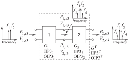
Figure \(\PageIndex{2}\): Cascade of two stages used in determining the third-order intercept point of a cascaded system.

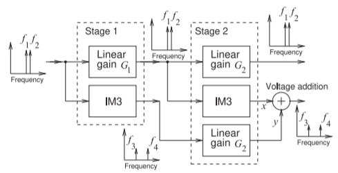
Figure \(\PageIndex{3}\): Signal flow for calculating the intermodulation distortion in the cascade of two stages.

is assumed, in that the \(\text{IM3}\) produces from each stage in the cascade add in phase. The other method is the unorganized cascade intercept method in which the phases of \(\text{IM3}\) produce by each stage are unknown, and assumes that the most likely overall \(\text{IM3}\) distortion will be obtained by assuming a random phase relationship of the \(\text{IM3}\) contributions.

The third-order intercept point, \(\text{IP3}\), is determined by extrapolating the small signal gain and \(\text{IM3}\) responses. Since \(\text{IM3}\) is small, the signal flow in the two-stage system is as shown in Figure \(\PageIndex{3}\). One path in the flow linearly amplifies the input two-tone signal in Stages \(1\) and \(2\). The third-order nonlinearity of Stage \(1\) creates low-level \(\text{IM3}\) that is linearly amplified by the second stage. A second set of \(\text{IM3}\) signals is produced by the \(\text{IM3}\) of the second stage operating on the two-tone signal amplified by Stage \(1\). The voltages of the two \(\text{IM3}\) signals add constructively. A complication is that the phases of the two \(\text{IM3}\) signals, at \(x\) and \(y\), are not known. This leads to two approaches to estimating of the overall distortion.

Organized Cascade Intercept Method

The worst-case situation is that the \(\text{IM3}\) voltages at \(x\) and \(y\) are in phase so that the voltages add. Then the total \(\text{IM3}\) distortion is obtained by adding the IM3 voltages generated from each stage. Determining total \(\text{OIP3}\), \(\text{OIP3}^{\text{T}}\) is the inverse problem. This cannot be solved precisely, but a good estimate for \(\text{OIP3}^{\text{T}}\) is obtained from [3, 4]

\[\label{eq:10}(\text{OIP3}^{\text{T}})^{-\frac{1}{2}}\approx (G_{2}\text{OIP3}_{1})^{-\frac{1}{2}}+(\text{OIP3}_{2})^{-\frac{1}{2}} \]

Note that \(\text{OIP3}\) is a power and \(G\) is a power gain. Now the total gain of the cascade \(G^{T} = G_{1}G_{2}\), and since \(\text{OIP3}^{\text{T}} = G^{T}\text{IIP3}^{\text{T}}\), where \(\text{OIP3}^{\text{T}}\), the input intercept of the cascade, can be written

\[\label{eq:11}(\text{IIP3}^{\text{T}})^{-\frac{1}{2}}\approx (\text{IIP3}_{1})^{-\frac{1}{2}}+(\text{IIP3}_{2}/G_{1})^{-\frac{1}{2}} \]

Generalizing these results, for an \(m\)-stage cascade the overall \(\text{OIP3}\) is

\[\begin{align}(\text{OIP3}^{\text{T}})^{-\frac{1}{2}}&\approx (G_{m}\ldots G_{2}\text{OIP3}_{1})^{-\frac{1}{2}}+\ldots \left(G_{m}\text{OIP3}_{(m-1)}\right)^{-\frac{1}{2}}\nonumber \\ \label{eq:12} &\quad +(\text{OIP3}_{m})^{-\frac{1}{2}}\end{align} \]

Since \(\text{IIP3} = \text{OIP3}/G\), the general result for multiple cascaded stages can be written

\[\label{eq:13}\left(\frac{1}{\text{IIP3}^{\text{T}}}\right)^{\frac{1}{2}}\approx\left(\frac{1}{\text{IIP3}_{1}}\right)^{\frac{1}{2}}+\ldots \left(\frac{G_{(m-2)}\ldots G_{1}}{\text{IIP3}_{(m-1)}}\right)^{\frac{1}{2}}+\left(\frac{G_{(m-1)}\ldots G_{1}}{\text{IIP3}_{m}}\right)^{\frac{1}{2}} \]

The organized cascade intercept method often provides an overly conservative (i.e., far too low) estimate of \(\text{OIP3}^{\text{T}}\) and \(\text{IIP3}^{\text{T}}\) distortion.

Unorganized Cascade Intercept Method

If the phases of the stages are random (or perhaps unknown), then it is reasonable to add the powers of the distortion terms. This is an approximation as the \(\text{IM3}\) signals are still correlated, but this approach has been found to provide a useful measure in design, then

\[\label{eq:14}(\text{OIP3}^{\text{T}})^{-1}\approx (G_{2}\text{OIP3}_{1})^{-1}+(\text{OIP3}_{2})^{-1} \]

and again \(\text{OIP3}\) is a power and \(G\) is a power gain. For an \(m\)-stage cascade with random \(\text{IM3}\) phase the total \(\text{OIP3}\), \(\text{OIP3}^{\text{T}}\), is obtained from

\[\label{eq:15}(\text{OIP3}^{\text{T}})^{-1}\approx (G_{m}\ldots G_{2}\text{OIP3}_{1})^{-1}+\ldots +(G_{2}\text{OIP3}_{(m-1)})^{-1}+(\text{OIP3}_{m})^{-1} \]

and the total \(\text{IIP3}\), \(\text{IIP3}^{\text{T}}\), is obtained from (since \(\text{IIP3} = \text{OIP3}/G)\)

\[\label{eq:16}\left(\frac{1}{\text{IIP3}^{\text{T}}}\right)\approx\left(\frac{1}{\text{IIP3}_{1}}\right)+\left(\frac{G_{1}}{\text{IIP3}_{2}}\right)+\ldots +\left(\frac{G_{(m-1)}\ldots G_{1}}{\text{IIP3}_{m}}\right) \]

Summary

The cascade intercept method has led to two sets of results for \(\text{IM3}\) distortion. The first, from the organized cascade intercept method, is the worst-case situation in which the \(\text{IM3}\) distortion of each stage combines in the worst possible way. This yielded the overall \(\text{IIP3}\) and \(\text{OIP3}\) results of Equations \(\eqref{eq:12}\) and \(\eqref{eq:13}\). The second, from the unorganized cascade intercept method, assumes that the phases of the \(\text{IM3}\) from each stage are randomly related, perhaps the best estimate that can be made without a circuit simulation. This yielded the overall \(\text{IIP3}\) and \(\text{OIP3}\) results of Equations \(\eqref{eq:15}\) and \(\eqref{eq:16}\).

It is interesting to speculate what would happen if the stages were designed so that the \(\text{IM3}\) contributions at \(x\) and \(y\) (referring to Figure \(\PageIndex{3}\)) of the first and second stages were \(180^{\circ}\) out of phase but with the same magnitude. If this could be done the \(\text{IM3}\) contributions at the output would be canceled. Indeed, it is possible to do this to a limited extent. The phase of the \(\text{IM3}\) signals depends on the signal level and so changes over the signal range. Careful design, and only when there is complete control over the design and integration of the stages, enables the IMD contributions to be partially canceled over a range of signal levels, as shown in Figure \(\PageIndex{4}\). This extends the dynamic range of the cascaded system, and the simple \(\text{OIP3}\) and \(\text{IIP3}\) metrics are not sufficient to capture this complexity.

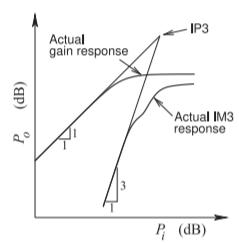
Figure \(\PageIndex{4}\): The gain and \(\text{IM3}\) responses of two cascaded stages showing the partial cancellation of the \(\text{IM3}\) response over a range of input signal levels.

Example \(\PageIndex{3}\): Intermodulation Distortion of a Two-Stage Amplifier

The first stage of a two-stage amplifier in a transmitter has a gain of \(G_{1} = 20\text{ dB}\) and an output third-order intercept point, \(\text{OIP3}_{1}\), of \(30\text{ dBm}\). The second stage has a gain of \(G_{2} = 20\text{ dB}\) and an \(\text{OIP3}\) of \(40\text{ dBm}\). Assume that the IMD contributions of each stage are in phase. What is the \(\text{OIP3}\) of the cascaded system?

Solution

Using the organized cascade intercept method, the total \(\text{OIP3}\), \(\text{OIP3}^{\text{T}}\), in milliwatts is obtained using Equation \(\eqref{eq:10}\)

\[\label{eq:17}\left(\text{OIP3}^{\text{T}}\right)^{-\frac{1}{2}}\approx\left(10^{(20/10)}10^{(30/10)}\right)^{-\frac{1}{2}}+\left(10^{(40/10)}\right)^{-\frac{1}{2}}=(10^{5})^{-\frac{1}{2}}+(10^{4})^{-\frac{1}{2}} \]

Thus

\[\label{eq:18}\text{OIP3}^{\text{T}}=5772\text{ mW}=37.6\text{ dBm} \]

This is the worst-case situation. It is worth comparing this to a calculation where the phases of the IMD contributions are unknown. Then, using Equation \(\eqref{eq:14}\),

\[\label{eq:19}\left(\text{OIP3}^{\text{T}}\right)^{-1}\approx\left(10^{(20/10)}10^{(30/10)}\right)^{-1}+\left(10^{(40/10)}\right)^{-1}=10^{5}+10^{4} \]

Thus

\[\label{eq:20}\text{OIP3}^{\text{T}}=9091\text{ mW}=39.6\text{ dBm} \]