7.3: Cascaded Module Design Using the Budget Method

Last updated
Save as PDF

Page ID: 46151

\( \newcommand{\vecs}[1]{\overset { \scriptstyle \rightharpoonup} {\mathbf{#1}} } \) \( \newcommand{\vecd}[1]{\overset{-\!-\!\rightharpoonup}{\vphantom{a}\smash {#1}}} \)\(\newcommand{\id}{\mathrm{id}}\) \( \newcommand{\Span}{\mathrm{span}}\) \( \newcommand{\kernel}{\mathrm{null}\,}\) \( \newcommand{\range}{\mathrm{range}\,}\) \( \newcommand{\RealPart}{\mathrm{Re}}\) \( \newcommand{\ImaginaryPart}{\mathrm{Im}}\) \( \newcommand{\Argument}{\mathrm{Arg}}\) \( \newcommand{\norm}[1]{\| #1 \|}\) \( \newcommand{\inner}[2]{\langle #1, #2 \rangle}\) \( \newcommand{\Span}{\mathrm{span}}\) \(\newcommand{\id}{\mathrm{id}}\) \( \newcommand{\Span}{\mathrm{span}}\) \( \newcommand{\kernel}{\mathrm{null}\,}\) \( \newcommand{\range}{\mathrm{range}\,}\) \( \newcommand{\RealPart}{\mathrm{Re}}\) \( \newcommand{\ImaginaryPart}{\mathrm{Im}}\) \( \newcommand{\Argument}{\mathrm{Arg}}\) \( \newcommand{\norm}[1]{\| #1 \|}\) \( \newcommand{\inner}[2]{\langle #1, #2 \rangle}\) \( \newcommand{\Span}{\mathrm{span}}\)\(\newcommand{\AA}{\unicode[.8,0]{x212B}}\)

The budget method is used to design RF cascade systems, particularly the design of receiver and transmitter cascaded systems, for specified gain, noise, and distortion. In the budget method, initial assignments of gain and noise performance are made to each stage in a cascade. This approach is based on the calculation of the total noise figure and gain of a system from the parameters of individual subsystem stages (see Section 4.3.1). This is coupled with the calculation of nonlinear distortion in cascaded stages (in Section 7.2), to calculate the spurious free dynamic range (SFDR) and make assignments for noise and distortion contributions of each stage [5]. The SFDR is related to the gain compression, noise, and nonlinear distortion metrics in Figure \(\PageIndex{1}\). The system optimization goal is, in general, to choose and adjust modules to maximize overall SFDR subject to the constraints of cost and availability of modules with the required attributes. For example, the gain of most amplifier modules can be adjusted and so change the

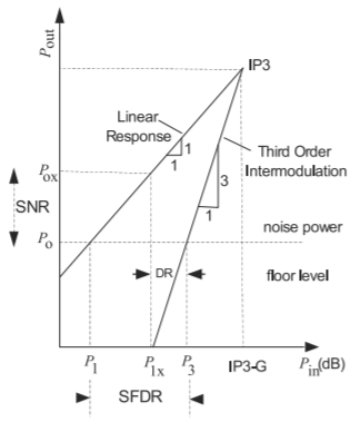
Figure \(\PageIndex{1}\): Output power versus input power of a stage or system. Extrapolations of the \(1:1\) linear response and the \(3:1\) third-order intermodulation response intersect at the \(\text{IP3}\) point. DR = dynamic range, SFDR = spurious free dynamic range, SNR = required minimum signal-to-noise ratio.

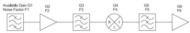
Figure \(\PageIndex{2}\): Cascade system for receive down converter or transmit up converter.

nonlinear distortion performance of amplifier stages. In the budget method the noise and nonlinear distortion metrics of each stage are set based on experience.

Considering the stages in the cascade shown in Figure \(\PageIndex{2}\), generally maximum gain is assigned to the first active stage, and so the first stage contributes the most to the system noise figure. However, as a consequence active devices in latter stages nearly always require significantly higher linearity performance than may be necessary to meet the system SFDR objective. Still the budget method is a systematic way to design a cascaded system. Experience can also be used in the budget assignments. For example, in transmitter cascade design the intent might be to provide as high an intercept as possible in the lower-frequency up-conversion stages. This approach is based on devices operating at lower frequencies having very good linearity and therefore being most cost effective in achieving high \(\text{IP3}\).