7.5: Case Study- High Dynamic Range Down-Converter Design

Last updated
Save as PDF

Page ID: 46153

\( \newcommand{\vecs}[1]{\overset { \scriptstyle \rightharpoonup} {\mathbf{#1}} } \) \( \newcommand{\vecd}[1]{\overset{-\!-\!\rightharpoonup}{\vphantom{a}\smash {#1}}} \)\(\newcommand{\id}{\mathrm{id}}\) \( \newcommand{\Span}{\mathrm{span}}\) \( \newcommand{\kernel}{\mathrm{null}\,}\) \( \newcommand{\range}{\mathrm{range}\,}\) \( \newcommand{\RealPart}{\mathrm{Re}}\) \( \newcommand{\ImaginaryPart}{\mathrm{Im}}\) \( \newcommand{\Argument}{\mathrm{Arg}}\) \( \newcommand{\norm}[1]{\| #1 \|}\) \( \newcommand{\inner}[2]{\langle #1, #2 \rangle}\) \( \newcommand{\Span}{\mathrm{span}}\) \(\newcommand{\id}{\mathrm{id}}\) \( \newcommand{\Span}{\mathrm{span}}\) \( \newcommand{\kernel}{\mathrm{null}\,}\) \( \newcommand{\range}{\mathrm{range}\,}\) \( \newcommand{\RealPart}{\mathrm{Re}}\) \( \newcommand{\ImaginaryPart}{\mathrm{Im}}\) \( \newcommand{\Argument}{\mathrm{Arg}}\) \( \newcommand{\norm}[1]{\| #1 \|}\) \( \newcommand{\inner}[2]{\langle #1, #2 \rangle}\) \( \newcommand{\Span}{\mathrm{span}}\)\(\newcommand{\AA}{\unicode[.8,0]{x212B}}\)

In this section a down-converter in a receiver is designed. With the architecture and modules chosen in the RF cascade, the only quantities that can be selected by the user are the gains of the amplifier stages. If adjusting the gains is not sufficient to meet system objectives, then it would be necessary to choose other modules or change the architecture.

7.5.1 Architecture

A down-converter with the architecture of Figure 7.3.2 is designed here considering the first four stages only and using the balanced contribution method for the initial stage assignment. The system operates at \(1.5\text{ GHz}\) with a first IF of \(250\text{ MHz}\) and an \(\text{IIP3}\) design target of \(0\text{ dBm}\) (i.e., \(\overline{\text{IIP3}}_{\text{dBm}}^{\text{T}} = 0\text{ dBm}\)) with a noise figure target of \(10\text{ dB}\) (i.e., \(\overline{\text{NF}}^{\text{T}} = 10\text{ dB}\)). The initial stage assignments for balanced noise and IMD contributions are shown in Table 7.4.1.

The stage assignments shown in Table 7.4.1 meet the target specifications exactly, with no single stage contributing any more than the required noise factor or nonlinearity (distortion) to meet the target. The LNA gain is low, permitting a significant reduction in required mixer \(\text{IP3}\). In an RF system usually the mixer has the limiting distortion performance so anything that can be done to reduce the linearity required for a mixer is advantageous. The noise figure of a mixer can also be high. With this in mind, the process of system cascade trade-off and selection of actual element parameters continues in the following sections. That is, assignment of balanced contributions to each stage is a good initial starting point. This is followed up with further optimization and trade-offs.

7.5.2 Design

Design proceeds with a selection of available modules for stages and continuous but limited variation of stage parameters (through bias control, for example). The following stages were chosen for the stages (see Figure 7.3.2): an MMIC amplifier for Stage \(2\) (NEC part \(\text{UPC2745}\)) and a MMIC mixer for Stage \(4\) (MCL part \(\text{SYM-2500}\)). Bandpass dielectric resonator filters were chosen for Stages \(1\) and \(3\). In particular, a tuned lumped-element Chebychev bandpass filter with \(0.1\text{ dB}\) ripple at \(1.5\text{ GHz}\) was used to provide settable loss in Stage \(3\) and this proved to be important in establishing balanced stage contributions and improved dynamic range. The continuous control parameters include controlling the mixer IMD contribution by changing the LNA gain (through bias control), changing the mixer \(\text{IIP3}\) (by varying the LO drive level), and retuning the Stage \(3\) filter. The noise and distortion contributions of stages with the initial stage assignment (from Table 7.4.1), initial measured performance, and optimized design are shown in Figures \(\PageIndex{1}\) and \(\PageIndex{2}\). Figure \(\PageIndex{3}\) depicts the dynamic range. Based on the balanced contribution method, the SFDR is \(109.5\text{ dB}\) normalized to a \(1\text{ Hz}\) bandwidth. The initial value provided by the devices selected is \(108\text{ dB}\). After appropriate trade-off and adjustable loss in Stage \(3\), the dynamic range achieved is \(111\text{ dB}\). Now the same system design could be achieved using the budget assignment initially, but with much greater design effort.

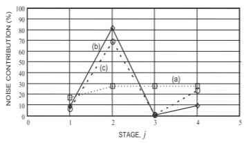
Figure \(\PageIndex{1}\): Noise figure contribution: (a) initial calculation of balanced noise figure contribution; (b) measured contributions of each stage using the initial assignments; and (c) final measured contributions after altering bias, filter loss, and mixer LO drive levels for improved dynamic range.

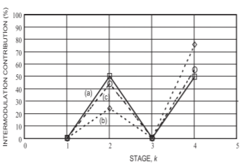
Figure \(\PageIndex{2}\): Input intercept (\(\text{IP3}\)) contribution: (a) initial calculation; (b) original measured contributions; and (c) final performance after alteration of bias, LO drive, and filter loss in Stage 3. Final settings in (c) led to the highest system dynamic range.

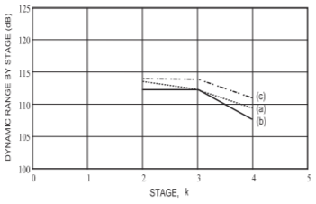
Figure \(\PageIndex{3}\): SFDR by stage: (a) initial assignment; (b) initial system performance after selection of modules but before optimization; and (c) final performance after setting bias, LO drive, and filter loss in Stage 3.