1.2: RF and Microwave Engineering

An RF signal is a signal that is coherently generated, radiated by a transmit antenna, propagated through air or space, collected by a receive antenna, and then amplified and information extracted. An RF circuit operates at the same frequency as the RF signal that is transmitted or received. That is, the frequency at which a circuit operates does not define that it is an RF circuit. The RF spectrum is part of the electromagnetic (EM) spectrum exploited by humans for communications. A broad categorization of the EM spectrum is shown in Table 1.1.1. Today radios operate from \(3\text{ Hz}\) to \(300\text{ GHz}\), although the upper end will increase as technology progresses.

Microwaves refers to the frequencies where the size of a circuit or structure is comparable to or greater than the wavelength of the EM signal. The division is arbitrary but if a circuit structure is greater than \(\frac{1}{20}\) of a wavelength, then most engineers would regard the circuit as being a microwave circuit. For now the microwave frequency range is generally taken as \(300\text{ MHz}\) to \(300\text{ GHz}\). At these frequencies distributed effects, sometimes called transmission line effects, must be considered.

One of the key characteristics distinguishing RF signals from infrared and visible light is that an RF signal can be generated with coherent phase, and information can be transmitted in both amplitude and phase variations of the RF signal. Such signals can be easily generated up to \(220\text{ GHz}\). The necessary hardware becomes progressively more expensive as frequency increases. The upper limit of radio frequencies is about \(300\text{ GHz}\) today, but the limit is extending slowly above this as technology progresses.

The RF bands are listed in Table \(\PageIndex{1}\) along with propagation modes and representative applications. The propagation of RF signals in free space follows one or more paths from a transmitter to a receiver at any frequency, with differences being in the size of the antennas needed to transmit and receive signals. The size of the necessary antenna is related to wavelength, with the typical dimensions ranging from a quarter of a wavelength to a few wavelengths if a reflector is used to focus the EM waves. On earth, and dependent on frequency, RF signals propagate through walls, diffract around objects, refract when the dielectric constant of the medium changes, and reflect from buildings and walls. The extent is dependent on frequency.

Above ground the propagation at RF is affected by atmospheric loss, by charge layers induced by solar radiation in the upper atmosphere, and by density variations in the air caused by heating as well as the thinning of air with height above the earth. The ionosphere is the uppermost part of the atmosphere, at \(60\) to \(90\text{ km}\), and is ionized by solar radiation, producing a reflective surface, called the D layer, to radio signals up to \(3\text{ GHz}\). The D layer weakens at night and most radio signals can then pass through this weakened layer. The E layer extends from \(90\) to \(120\text{ km}\) and is ionized by X-rays and extreme ultraviolet radiation, and the ionized regions, which reflect RF signals, form ionized clouds that last only a few hours. The F layer of the ionosphere extends from \(200\) to \(500\text{ km}\) and ionization in this layer is due to extreme ultraviolet radiation. Refraction results from this charged layer rather than reflection, as the charges are widely separated. At night the F layer results in what is called the skywave, which is the refraction of radio waves around the earth. At low frequencies a radio wave penetrates the earth’s surface and the wave can become trapped at the interface between two regions of different permittivity, the earth region and the air region. This radio wave is called the surface wave or ground wave.

Note

When a radio signal near \(60\text{ GHz}\) passes through air an oxygen molecule of two bound oxygen atoms vibrates and EM energy is transferred to the mechanical energy of vibration and thus heat.

Propagating RF signals in air are absorbed by molecules in the atmosphere primarily by molecular resonances such as the bending and stretching of bonds. This bending and stretching converts energy in the EM wave into vibrational energy of the molecules. The transmittance of radio signals versus frequency in dry air at an altitude of \(4.2\text{ km}\) is shown in Figure \(\PageIndex{1}\). The first molecular resonance encountered in dry air as frequency increases is the oxygen resonance, centered at \(60\text{ GHz}\), but below that the absorption in dry air is very small. Attenuation increases with higher water vapor pressure (with a resonance at \(22\text{ GHz}\)) and in rain. Within \(2\text{ GHz}\) of \(60\text{ GHz}\) a signal will not travel far, and this can be used to provide localized communication over a few meters as a local data link. Regions of low attenuation (i.e. high transmittance), are called windows and there are numerous low loss windows.

Band		Frequency wavelength	Propagation mode/applications
TLF	Tremendously low frequency	\(< 3\text{ Hz} > 100,000\text{ km}\)	Penetration of liquids and solids/Submarine communication
ELF	Extremely low frequency	\(3-30\text{ Hz}, 100,000-10,000\text{ km}\)	Penetration of liquids and solids/Submarine communication
SLF	Super low frequency	\(30-300\text{ Hz}, 10,000-1,000\text{ km}\)	Penetration of liquids and solids/Submarine communication
ULF	Ultra low frequency	\(300-3,000\text{ Hz}, 1,000-100\text{ km}\)	Penetration of liquids and solids/Submarine communication; communication within mines
VLF	Very low frequency	\(3-30\text{ kHz}, 100-10\text{ km}\)	Guided wave trapped between the earth and the ionosphere/Navigation, geophysics
LF	Low frequency	\(30-300\text{ kHz}, 10-1\text{ km}\)	Guided wave between the earth and the ionosphere’s D layer; surface waves, building penetration/Navigation, AM broadcast, amateur radio, time signals, RFID
MF	Medium frequency	\(300-3,000\text{ kHz}, 1000-100\text{ m}\)	Surface wave, building penetration; day time: guided wave between the earth and the ionosphere’s D layer; night time: sky wave/AM broadcast
HF	High frequency	\(3-30\text{ MHz}, 100-10\text{ m}\)	Sky wave, building penetration/shortwave broadcast, over-the-horizon radar, RFID, amateur radio, marine and mobile telephony
VHF	Very high frequency	\(30-300\text{ MHz}, 10-1\text{ m}\)	Line of sight, building penetration; up to \(80\text{ MHz}\), skywave during periods of high sunspot activity/FM and TV broadcast, weather radio, line-of-sight aircraft communications
UHF	Ultra high frequency	\(300-3000\text{ MHz}, 10-1\text{ cm}\)	Line of sight, building penetration; sometimes tropospheric ducting/1G–4G cellular communications, RFID, microwave ovens, radio astronomy, satellite-based navigation
SHF	Super high frequency	\(3-30\text{ GHz}, 10-1\text{ cm}\)	Line of sight/5G cellular communications, Radio astronomy, point-to-point communications, wireless local area networks, radar
EHF	Extremely high frequency	\(30-300\text{ GHz}, 10-1\text{ mm}\)	Line of sight/5G cellular communications, Astronomy, remote sensing, point-to-point and satellite communications
THF	Terahertz or tremendously high frequency	\(300-3,000\text{ GHz}, 1,000-100\:\mu\text{m}\)	Line of sight /Spectroscopy, imaging

Table \(\PageIndex{1}\): Radio frequency bands, primary propagation mechanisms, and selected applications.

RF signals diffract and so can bend around structures and penetrate into valleys. The ability to diffract reduces with increasing frequency. However, as frequency increases the size of antennas decreases and the capacity to carry information increases. A very good compromise for mobile communications is at UHF, \(300\text{ MHz}\) to \(4\text{ GHz}\), where antennas are of convenient size and there is a good ability to diffract around objects and even penetrate walls. This choice can be seen with 1G–4G cellular communication systems operating in several bands from \(450\text{ MHz}\) to \(3.6\text{ GHz}\) where antennas do not dominate the size of the handset, and the ability to receive calls within buildings and without line of sight to the base station is well known.

RF bands have been further divided for particular applications. The

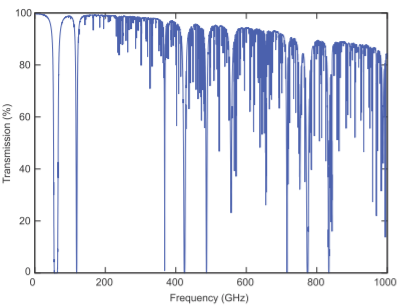
Figure \(\PageIndex{1}\): Atmospheric transmission at Mauna Kea, with a height of \(4.2\text{ km}\), on the Island of Hawaii where the atmospheric pressure is \(60\%\) of that at sea level and the air is dry with a precipitable water vapor level of \(0.001\text{ mm}\). After [5].

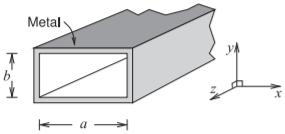
Figure \(\PageIndex{2}\): Rectangular waveguide with internal dimensions of \(a\) and \(b\). Usually \(a ≈ b\). The EM waves are confined within the four metal walls and propagate in the \(±z\) direction. Little current flows in the waveguide walls and so resistive losses are small. Compared to coaxial lines rectangular waveguides have very low loss.

frequency bands for radar are shown in Table 1.3.1. The L, S, and C bands are referred to as having octave bandwidths, as the upper frequency of a band is twice the lower frequency. The other bands are half-octave bands, as the upper frequency limit is approximately 50% higher than the lower frequency limit. The same letter band designations are used by other standards. The most important alternative band designation is for the waveguide bands. These bands refer to the useful range of operation of a rectangular waveguide, which is a rectangular tube that confines a propagating signal within four conducting walls (see Figure \(\PageIndex{2}\)). The waveguide bands are shown in Table 1.3.2 with the conventional letter designation of bands and standardized waveguide dimensions. Compared to coaxial lines rectangular waveguides have very low loss.\(^{1}\)

Footnotes

[1] A semirigid coaxial line with an outer conductor diameter of \(3.5\text{ mm}\) has a loss at \(10\text{ GHz}\) of \(0.5\text{ db/m}\) while an X-band waveguide has a loss of \(0.1\text{ dB/m}\). At \(100\text{ GHz}\) a \(1\text{ mm}\)-diameter coaxial line has a loss of \(12.5\text{ dB/m}\) compared to \(2.5\text{ dB/m}\) loss for a W-band waveguide.