
1.3: Communication Over Distance
- Page ID
- 41165

Communicating using EM signals has been an integral part of society since the transmission of the first telegraph signals over wires in the mid 19th century [7]. This development derived from an understanding of magnetic induction based on the experiments of Faraday in 1831 [8] in which he investigated the relationship of magnetic fields and currents. This work of Faraday is now known as Faraday’s law, or Faraday’s law of induction. It was one of four key laws developed between 1820 and 1835 that described the interaction of static fields and of static fields with currents. These four
| Band | Frequency Range |
|---|---|
| \(\text{L}\) "long" | \(1-2\text{ GHz}\) |
| \(\text{S}\) "short" | \(2-4\text{ GHz}\) |
| \(\text{C}\) "compromise" | \(4-8\text{ GHz}\) |
| \(\text{X}\) "extended" | \(8-12\text{ GHz}\) |
| \(\text{K}_{u}\) "kurtz under" | \(12-18\text{ GHz}\) |
| \(\text{K}\) "kurtz" (short in German) | \(18-27\text{ GHz}\) |
| \(\text{K}_{a}\) "kurtz above" | \(27-40\text{ GHz}\) |
| \(\text{V}\) | \(40-75\text{ GHz}\) |
| \(\text{W}\) | \(75-110\text{ GHz}\) |
| \(\text{F}\) | \(90-140\text{ GHz}\) |
| \(\text{D}\) | \(110-170\text{ GHz}\) |
| \(\text{mm}\) | \(110-300\text{ GHz}\) |
Table \(\PageIndex{1}\): IEEE radar bands [6]. The mm band designation is also used when the intent is to convey general information above \(30\text{ GHz}\).
Note
In Table \(\PageIndex{2}\) the waveguide dimensions are specified in inches (use \(25.4\text{ mm/inch}\) to convert to \(\text{mm}\)). The number in the WR designation is the long internal dimension of the waveguide in hundredths of an inch. The EIA is the U.S.-based Electronics Industry Association. Note that the radar band (see Table \(\PageIndex{1}\)) and waveguide band designations do not necessarily coincide.
| Band | EIA Waveguide Band | Operating Frequency (\(\text{GHz}\)) | Internal Dimensions (\(a\times b\), inches) |
|---|---|---|---|
| \(\text{R}\) | WR-430 | \(1.70-2.60\) | \(4.300\times 2.150\) |
| \(\text{D}\) | WR-340 | \(2.20-3.30\) | \(3.400\times 1.700\) |
| \(\text{S}\) | WR-284 | \(2.60-3.95\) | \(2.840\times 1.340\) |
| \(\text{E}\) | WR-229 | \(3.30-4.90\) | \(2.290\times 1.150\) |
| \(\text{G}\) | WR-187 | \(3.95-5.85\) | \(1.872\times 0.872\) |
| \(\text{F}\) | WR-159 | \(4.90-7.05\) | \(1.590\times 0.795\) |
| \(\text{C}\) | WR-137 | \(5.85-8.20\) | \(1.372\times 0.622\) |
| \(\text{H}\) | WR-112 | \(7.05-10.00\) | \(1.122\times 0.497\) |
| \(\text{X}\) | WR-90 | \(8.2-12.4\) | \(0.900\times 0.400\) |
| \(\text{Ku}\) | WR-62 | \(12.4-18.0\) | \(0.622\times 0.311\) |
| \(\text{K}\) | WR-51 | \(15.0-22.0\) | \(0.510\times 0.255\) |
| \(\text{K}\) | WR-42 | \(18.0-26.5\) | \(0.420\times 0.170\) |
| \(\text{Ka}\) | WR-28 | \(26.5-40.0\) | \(0.280\times 0.140\) |
| \(\text{Q}\) | WR-22 | \(33-50\) | \(0.224\times 0.112\) |
| \(\text{U}\) | WR-19 | \(40-60\) | \(0.188\times 0.094\) |
| \(\text{V}\) | WR-15 | \(50-75\) | \(0.148\times 0.074\) |
| \(\text{E}\) | WR-12 | \(60-90\) | \(0.122\times 0.061\) |
| \(\text{W}\) | WR-10 | \(75-110\) | \(0.100\times 0.050\) |
| \(\text{F}\) | WR-8 | \(90-140\) | \(0.080\times 0.040\) |
| \(\text{D}\) | WR-6 | \(110-170\) | \(0.0650\times 0.0325\) |
| \(\text{G}\) | WR-5 | \(140-220\) | \(0.0510\times 0.0255\) |
Table \(\PageIndex{2}\): Selected waveguide bands with operating frequencies and internal dimensions (refer to Figure 1.2.2).
laws are the Biot–Savart law (developed around 1820), Ampere’s law (1826), Faraday’s law (1831), and Gauss’s law (1835). These are all static laws and do not describe propagating fields.
1.3.1 Electromagnetic Fields
We now know that there are two components of the EM field, the electric field, \(E\), with units of volts per meter (\(\text{V/m}\)), and the magnetic field, \(H\), with units of amperes per meter (\(\text{A/m}\)). \(E\) and \(H\) fields together describe the force between charges. There are also two flux quantities that are necessary to understand the interactions between these fields and vacuum or matter. The first is \(D\), the electric flux density, with units of coulombs per square meter (\(\text{C/m}^{2}\)), and the other is \(B\), the magnetic flux density, with units of teslas (\(\text{T}\)). \(B\) and \(H\), and \(D\) and \(E\), are related to each other by the properties of the medium, which are embodied in the quantities \(\mu\) and \(\varepsilon\) (with the caligraphic letter, e.g. \(\mathcal{B}\), denoting a time-domain quantity):
\[\label{eq:1}\overline{\mathcal{B}}=\mu\overline{\mathcal{H}} \]
\[\label{eq:2}\overline{\mathcal{D}}=\varepsilon\overline{\mathcal{E}} \]
where the over bar denotes a vector quantity, and \(\mu\) is called the permeability of the medium and describes the ability to store magnetic energy in a region. The permeability in free space (or vacuum) is denoted \(\mu_{0}=4\pi\times 10^{-7}\text{ H/m}\) and the magnetic flux and magnetic field are related as
\[\label{eq:3}\overline{\mathcal{B}}=\mu_{0}\overline{\mathcal{H}} \]
The other material quantity is the permittivity, \(\varepsilon\), which describes the ability to store energy in a volume and in a vacuum
\[\label{eq:4}\overline{\mathcal{D}}=\varepsilon_{0}\overline{\mathcal{E}} \]
where \(\varepsilon_{0} = 8.854\times 10^{-12}\text{ F/m}\) is the permittivity of a vacuum. The relative permittivity, \(\varepsilon_{r}\), is the ratio the permittivity of a material to that of vacuum:
\[\label{eq:5}\varepsilon_{r}=\varepsilon /\varepsilon_{0} \]
Similarly, the relative permeability, \(\mu_{r}\), refers to the ratio of permeability of a material to its value in a vacuum:
\[\label{eq:6}\mu_{r}=\mu /\mu_{0} \]
1.3.2 Biot-Savart Law
The Biot–Savart law relates current to magnetic field as, see Figure \(\PageIndex{1}\),
\[\label{eq:7}d\overline{H} = \frac{Id\ell\times\hat{a}_{R}}{4\pi R^{2}} \]
which has the units of amperes per meter in the SI system. In Equation \(\eqref{eq:7}\) \(d\overline{H}\) is the incremental static \(H\) field, \(I\) is current, \(d\ell\) is the vector of the length of a filament of current \(I\), \(\hat{a}_{R}\) is the unit vector in the direction from the current filament to the magnetic field, and \(R\) is the distance between the filament and the magnetic field. The \(d\overline{H}\) field is directed at right angles to \(\hat{a}_{R}\) and the current filament. So Equation \(\eqref{eq:7}\) says that a filament of current produces a magnetic field at a point. The total magnetic field from a current on a wire or surface can be found by modeling the wire or surface as a number of current filaments, and the total magnetic field at a point is obtained by integrating the contributions from each filament.
1.3.3 Faraday's Law of Induction
Faraday’s law relates a time-varying magnetic field to an induced voltage drop, \(V\), around a closed path, which is now understood to be \(\oint_{\ell}\overline{\mathcal{E}}\cdot d\ell\), that is, the closed contour integral of the electric field,
\[\label{eq:8}V=\oint_{\ell}\overline{\mathcal{E}}\cdot d\ell = -\oint_{s}\frac{\partial\overline{\mathcal{B}}}{\partial t}\cdot d\text{s} \]
and this has the units of volts in the SI unit system. The operation described in Equation \(\eqref{eq:8}\) is illustrated in Figure \(\PageIndex{2}\).
1.3.4 Ampere's Circuital Law
Ampere’s circuital law, often called just Ampere’s law, relates direct current and the static magnetic field \(\overline{\mathcal{H}}\). The relationship is based on Figure \(\PageIndex{3}\) and Ampere’s circuital law is
\[\label{eq:9}\oint_{\ell}\overline{H}\cdot d\ell = I_{\text{enclosed}} \]
That is, the integral of the magnetic field around a loop is equal to the current enclosed by the loop. Using symmetry, the magnitude of the magnetic field at a distance \(r\) from the center of the wire shown in Figure \(\PageIndex{3}\) is
\[\label{eq:10}H=|I|/(2\pi r) \]
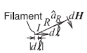
Figure \(\PageIndex{1}\): Diagram illustrating the Biot-Savart law. The law relates a static filament of current to the incremental \(H\) field at a distance.
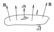
Figure \(\PageIndex{2}\): Diagram illustrating Faraday’s law. The contour \(\ell\) encloses the surface.
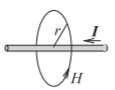
Figure \(\PageIndex{3}\): Diagram illustrating Ampere’s law. Ampere’s law relates the current, \(I\), on a wire to the magnetic field around it, \(H\).
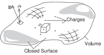
Figure \(\PageIndex{4}\): Diagram illustrating Gauss’s law. Charges are distributed in the volume enclosed by the closed surface. An incremental area is described by the vector \(d\mathbf{S}\), which is normal to the surface and whose magnitude is the area of the incremental area.
1.3.5 Gauss's Law
The final static EM law is Gauss’s law, which relates the static electric flux density vector, \(\overline{\mathcal{D}}\), to charge. With reference to Figure \(\PageIndex{4}\), Gauss’s law in integral form is
\[\label{eq:11}\oint_{s}\overline{D}\cdot d\text{s}=\int_{v}\rho_{v}\cdot dv=Q_{\text{enclosed}} \]
This states that the integral of the electric flux vector, \(\overline{D}\), over a closed surface is equal to the total charge enclosed by the surface, \(Q_{\text{enclosed}}\).
1.3.6 Gauss's Law of Magnetism
Gauss’s law of magnetism parallels Gauss’s law which now applies to magnetic fields. In integral form the law is
\[\label{eq:12}\oint_{s}\overline{B}\cdot d\text{s}=0 \]
This states that the integral of the magnetic flux vector, \(\overline{D}\), over a closed surface is zero reflecting the fact that magnetic charges do not exist.
1.3.7 Telegraph
With the static field laws established, the stage was set to begin the development of the transmission of EM signals over wires. While traveling by ship back to the United States from Europe in 1832, Samuel Morse learned of Faraday’s experiments and conceived of an EM telegraph. He sought out partners in Leonard Gale, a professor of science at New York University, and Alfred Vail, “skilled in the mechanical arts,” who constructed the telegraph models used in their experiments. In 1835 this collaboration led to an experimental version transmitting a signal over \(16\text{ km}\) of wire. Morse was not
| Symbol | Code |
|---|---|
| \(1\) | .---- |
| \(2\) | ..--- |
| \(3\) | ...-- |
| \(4\) | ....- |
| \(5\) | ..... |
| \(6\) | -.... |
| \(7\) | --... |
| \(8\) | ---.. |
| \(9\) | ----. |
| \(0\) | ----- |
| \(\text{A}\) | . - |
| \(\text{B}\) | -... |
| \(\text{C}\) | -.-. |
| \(\text{D}\) | -.. |
| \(\text{E}\) | . |
| \(\text{F}\) | ..-. |
| \(\text{G}\) | --. |
| \(\text{H}\) | .... |
| \(\text{I}\) | . . |
| \(\text{J}\) | .--- |
| \(\text{K}\) | -.- |
| \(\text{L}\) | .-.. |
| \(\text{M}\) | - - |
| \(\text{N}\) | - . |
| \(\text{O}\) | --- |
| \(\text{P}\) | .--. |
| \(\text{Q}\) | --.- |
| \(\text{R}\) | .-. |
| \(\text{S}\) | ... |
| \(\text{T}\) | - |
| \(\text{U}\) | ..- |
| \(\text{V}\) | ...- |
| \(\text{W}\) | .-- |
| \(\text{X}\) | -..- |
| \(\text{Y}\) | -.-- |
| \(\text{Z}\) | --.. |
Table \(\PageIndex{3}\): International Morse code.
alone in imagining an EM telegraph, and in 1837 Charles Wheatstone opened the first commercial telegraph line between London and Camden Town, England, a distance of \(2.4\text{ km}\). Subsequently, in 1844, Morse designed and developed a line to connect Washington, DC, and Baltimore, Maryland. This culminated in the first public transmission on May 24, 1844, when Morse sent a telegraph message from the Capitol in Washington to Baltimore. This event is recognized as the birth of communication over distance using wires. This rapid pace of transition from basic research into electromagnetism (Faraday’s experiment) to a fielded transmission system has been repeated many times in the evolution of wired and wireless communication technology.
The early telegraph systems used EM induction and multicell batteries that were switched in and out of circuit with the long telegraph wire and so created pulses of current. We now know that these current pulses created propagating magnetic fields that were guided by the wires and were accompanied by electric fields. In 1840 Morse applied for a U.S. patent for “Improvement in the Mode of Communicating Information by Signals by the Application of Electro-Magnetism Telegraph,” which described “lightning wires” and “Morse code.” By 1854, \(37,000\text{ km}\) of telegraph wire crossed the United States, and this had a profound effect on the development of the country. Railroads made early extensive use of telegraph and a new industry was created. In the United States the telegraph industry was dominated by Western Union, which became one of the largest companies in the world. Just as with telegraph, the history of wired and wireless communication has been shaped by politics, business interests, market risk, entrepreneurship, patent ownership, and patent litigation as much as by the technology itself.
The first telegraph signals were just short bursts and slightly longer bursts of noise using Morse code in which sequences of dots, dashes, and pauses represent numbers and letters (see Table \(\PageIndex{3}\)).\(^{1}\) The speed of transmission was determined by an operator’s ability to key and recognize the codes. Information transfer using EM signals in the late 19th century was therefore about \(5\) bits per second (bits/s). Morse achieved \(10\) words per minute.
1.3.8 The Origins of Radio
In the 1850s Morse began to experiment with wireless transmission, but this was still based on the principle of conduction. He used a flowing river, which as is now known is a medium rich with ions, to carry the charge. On one side of the river he set up a series connection of a metal plate, a battery, a Morse key, and a second metal plate. This formed the transmitter circuit. The metal plates were inserted into the water and separated by a distance considerably greater than the width of the river. On the other side of the river, metal plates were placed directly opposite the transmitter plates and this second set of plates was connected by a wire to a galvanometer in series. This formed the receive circuit, and electric pulses established by the transmitter resulted in the charge being transferred across the river by conduction and the pulses subsequently detected by the galvanometer. This was the first wireless transmission using electromagnetism, but it was not radio.
Morse relied entirely on conduction to achieve wireless transmission and it is now known that we need alternating electric and magnetic fields to propagate information over distance without charge carriers. The next steps in the progress to radio were experiments in induction. These culminated in an experiment by Loomis who in 1866 sent the first aerial wireless signals using kites flown by copper wires [9]. The transmitter kite had a Morse key at the ground end and an electric potential would have been developed between the ground and the kite itself. Closing the key resulted in current flow along the wire and this created a magnetic field that spread out and induced a current in the receive kite and this was detected by a galvanometer. However, not much of an electric field is produced and an EM wave is not transmitted. As such, the range of this system is very limited. Practical wireless communication requires an EM wave at a high-enough frequency that it can be efficiently generated by short wires.
1.3.9 Maxwell's Equations
The essential next step in the invention of radio was the development of Maxwell’s equations in 1861. Before Maxwell’s equations were postulated, several static EM laws were known. These are the Biot–Savart law, Ampere’s circuital law, Gauss’s law, and Faraday’s law. Taken together they cannot describe the propagation of EM signals, but they can be derived from Maxwell’s equations. Maxwell’s equations cannot be derived from the static electric and magnetic field laws. Maxwell’s equations embody additional insight relating spatial derivatives to time derivatives, which leads to a description of propagating fields. Maxwell’s equations are
\[\label{eq:13}\nabla\times\overline{\mathcal{E}}=-\frac{\partial\overline{\mathcal{B}}}{\partial t}-\overline{\mathcal{M}} \]
\[\label{eq:14}\nabla\cdot\overline{\mathcal{D}}=\rho_{V} \]
\[\label{eq:15}\nabla\times\overline{\mathcal{H}}=\frac{\partial\overline{\mathcal{D}}}{\partial t}+ \overline{\mathcal{J}} \]
\[\label{eq:16}\nabla\cdot\overline{\mathcal{B}}=\rho_{mV} \]
Several of the quantities in Maxwell’s equation have already been introduced, but now the electric and magnetic fields are in vector form. The other quantities in Equations \(\eqref{eq:13}\)–\(\eqref{eq:16}\) are
- \(\overline{\mathcal{J}}\), the electric current density, with units of amperes per square meter (\(\text{A/m}^{2}\));
- \(\rho_{V}\), the electric charge density, with units of coulombs per cubic meter (\(\text{C/m}^{3}\));
- \(\rho_{mV}\), the magnetic charge density, with units of webers per cubic meter (\(\text{Wb/m}^{3}\)); and
- \(\overline{\mathcal{M}}\), the magnetic current density, with units of volts per square meter (\(\text{V/m}^{2}\)).
Magnetic charges do not exist, but their introduction through the magnetic charge density, \(\rho_{mV}\), and the magnetic current density, \(\overline{\mathcal{M}}\), introduce an aesthetically appealing symmetry to Maxwell’s equations. Maxwell’s equations are differential equations, and as with most differential equations, their solution is obtained with particular boundary conditions, which in radio engineering are imposed by conductors. Electric conductors (i.e., electric walls) support electric charges and hence electric current. By analogy, magnetic walls support magnetic charges and magnetic currents. Magnetic walls also provide boundary conditions to be used in the solution of Maxwell’s equations. The notion of magnetic walls is important in RF and microwave engineering, as they are approximated by the boundary between two dielectrics of different permittivity. The greater the difference in permittivity, the more closely the boundary approximates a magnetic wall.
Maxwell’s equations are fundamental properties and there is no underlying theory, so they must be accepted “as is,” but they have been verified in countless experiments. Maxwell’s equations have three types of derivatives. First, there is the time derivative, \(\partial /\partial t\). Then there are two spatial derivatives, \(\nabla\times\), called curl, capturing the way a field circulates spatially (or the amount that it curls up on itself), and \(\nabla\cdot\), called the div operator, describing the spreading-out of a field. In rectangular coordinates, curl, \(\nabla\times\), describes how much a field circles around the \(x\), \(y\), and \(z\) axes. That is, the curl describes how a field circulates on itself. So Equation \(\eqref{eq:13}\) relates the amount an electric field circulates on itself to changes of the \(B\) field in time. So a spatial derivative of electric fields is related to a time derivative of the magnetic field. Also in Equation \(\eqref{eq:15}\) the spatial derivative of the magnetic field is related to the time derivative of the electric field. These are the key elements that result in self-sustaining propagation.
Div, \(\nabla\cdot\), describes how a field spreads out from a point. So the presence of net electric charge (say, on a conductor) will result in the electric field spreading out from a point (see Equation \(\eqref{eq:14}\)). In contrast, the magnetic field (Equation \(\eqref{eq:16}\)) can never diverge from a point, which is a result of magnetic charges not existing (except when the magnetic wall approximation is used).
How fast a field varies with time, \(\partial\overline{\mathcal{B}}/\partial t\) and \(\partial\overline{\mathcal{D}}/\partial t\), depends on frequency. The more interesting property is how fast a field can change spatially, \(\nabla\times\overline{\mathcal{E}}\) and \(\nabla\times\overline{\mathcal{H}}\)—this depends on wavelength relative to geometry. So if the cross-sectional dimensions of a transmission line are less than a wavelength (\(\lambda /2\) or \(\lambda /4\) in different circumstances), then it will be impossible for the fields to curl up on themselves and so there will be only one solution (with no or minimal spatial variation of the \(E\) and \(H\) fields) or, in some cases, no solution to Maxwell’s equations.
1.3.10 Transmission of Radio Signals
Now the discussion returns to the technological development of radio. About the same time as Loomis’s induction experiments in 1864, James Maxwell [10] laid the foundations of modern EM theory in 1861 [11]. Maxwell theorized that electric and magnetic fields are different manifestations of the same phenomenon. The revolutionary conclusion was that if they are time varying, then they would travel through space as a wave. This insight was accepted almost immediately by many people and initiated a large number of endeavors. The period of 1875 to 1900 was a time of tremendous innovation in wireless communication.
On November 22, 1875, Edison observed EM sparks. Previously sparks were considered to be an induction phenomenon, but Edison thought that he was producing a new kind of force, which he called the etheric force. He believed that this would enable communication without wires. To put this in context, the telegraph was invented in the 1830s and the telephone was invented in 1876.
The next stage leading to radio was orchestrated by D. E. Hughes beginning in 1879. Hughes experimented with a spark gap and reasoned that in the gap there was a rapidly alternating current and not a constant current as others of his time believed. The electric oscillator was born. The spark gap transmitter was augmented with a clockwork mechanism to interrupt the transmitter circuit and produce pulsed radio signals. He used a telephone as a receiver and walked around London and detected the transmitted signals over distance. Hughes noted that he had good reception at \(180\text{ feet}\). Hughes publicly demonstrated his “radio” in 1870 to the Royal Society, but the eminent scientists of the society determined that the effect was simply due to induction. This discouraged Hughes from continuing. However, Hughes has a legitimate claim to having invented radio, mobile digital radio at that, and probably was transmitting pulses on a \(100\text{ kHz}\) carrier. In Hugeness’s radio the RF carrier was produced by the spark gap oscillator and the information was coded as pulses. It was a small leap to a Morse key-based system.
The invention of practical radio can be attributed to many people, beginning with Heinrich Hertz, who in the period from 1885 to 1889 successfully verified the essential prediction of Maxwell’s equations that EM energy could propagate through the atmosphere. Hertz was much more thorough than Hughes and his results were widely accepted. In 1891 Tesla developed what is now called the Tesla coil, which is a transformer with a primary and a secondary coil, one inside the other. When one of the coils was excited by an alternating signal, a large voltage was produced across the terminals of the other coil. Tesla pursued the application of his coils to radio and realized that the coils could be tuned so that the resulting resonance greatly amplified a radio signal.
The next milestone was the establishment of the first practical radio system by Marconi, with experiments beginning in 1894. Oscillations were produced in a spark gap, which were amplified by a Tesla coil. The work culminated in the transmission of telegraph signals across the Atlantic (from Ireland to Canada) by Marconi in 1901. In 1904, crystal radio kits to detect wireless telegraph signals could be readily purchased.
Spark gap transmitters could only send pulses of noise and not voice. One generator that could be amplitude modulated was an alternator. At the end
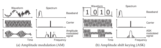
Figure \(\PageIndex{5}\): Waveform and spectra of simple modulation schemes. The modulating signal, at the top in (a) and (b), is also called the baseband signal.
of the 19th century, readily available alternators produced a \(60\text{ Hz}\) signal. Reginald Resplendent attempted to make a higher-frequency alternator and the best he achieved operated at \(1\text{ kHz}\). Resplendent realized that Maxwell’s equations indicated that radiation increased dramatically with frequency and so he needed a much-higher-frequency signal source. Under contract, General Electric developed a \(2\text{ kW}\), \(100\text{ kHz}\) alternator designed by Ernst Alexanderson. With this alternator, the first radio communication of voice occurred on December 23, 1900, in a transmission by Fessenden from an island in the Potomac River, near Washington, DC. Then on December 24, 1906, Fessenden transmitted voice from Massachusetts to ships hundreds of miles away in the Atlantic Ocean. This milestone is regarded as the beginning of the radio era.
Marconi subsequently purchased \(50\) and \(200\text{ kW}\) Alexanderson alternators for his trans-Atlantic transmissions. Marconi was a great integrator of ideas, with particular achievements being the design of transmitting and receiving antennas that could be tuned to a particular frequency and the development of a coherer to improve detection of a signal.
1.3.11 Early Radio
Radio works by superimposing relatively slowly varying information, at what is called the baseband frequency, on a carrier sinusoid by varying the amplitude and/or phase of the sinusoid. Early radio systems were based on modulating an oscillating carrier either by pulsing the carrier (using for example Morse code)—this modulation scheme is called amplitude shift keying (ASK)—or by varying the amplitude of the carrier, i.e. amplitude modulation (AM), in the case of analog, usually voice, transmission. The waveforms and spectra of these modulation schemes are shown in Figure \(\PageIndex{5}\). The information is contained in the baseband signal, which is also called the modulating signal. The spectrum of the baseband signal extends to DC or perhaps down to where it rolls off at a low frequency. The carrier is a single sinewave and contains no information. The amplitude of the carrier is varied by the baseband signal to produce the modulated signal. In general, there are many cycles of the carrier relative to variations of the baseband signal so that the bandwidth of the modulated signal is relatively small compared to the frequency of the carrier.
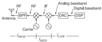
Figure \(\PageIndex{6}\): A simple transmitter with low, \(f_{\text{LOW}}\), medium, \(f_{\text{MED}}\), and high frequency, \(f_{\text{HIGH}}\), sections. The mixers can be idealized as multipliers, shown as circles with crosses, that boost the frequency of the input baseband or IF signal by the frequency of the carrier.
AM and ASK radios are narrowband communication systems (they use a small portion of the EM spectrum), so to avoid interference with other radios it is necessary to search for an open part of the spectrum to place the carrier signal. In the decade of the 1900s there was little organization and a listener needed to search to find the desired transmission. The technology of the day necessitated this anyway, as the carrier would drift around by \(10\%\) or so since it was then not possible to build a stable oscillator. It was not until the Titanic sinking in 1912 that regulation was imposed on the wireless industry. Investigations of the Titanic sinking concluded that most of the lives lost would have been saved if a nearby ship had been monitoring its radio channels and if the frequency of the emergency channel was fixed. However, a second ship, but not close enough, did respond to Titanic’s “SOS” signal. A result of the investigations was the Service Regulations of the 1912 London International Radiotelegraph Convention.
These early regulations were fairly liberal and radio stations were allowed to use radio wavelengths of their own choosing, but restricted to four broad bands: a single band at \(1500\text{ kHz}\) for amateurs; \(187.5\) to \(500\text{ kHz}\), appropriated primarily for government use; below \(187.5\text{ kHz}\) for commercial use, and \(500\text{ kHz}\) to \(1500\text{ kHz}\), also a commercial band. Subsequent years saw more stringent assignment of narrow spectral bands and the assignment of channels. The standards and regulatory environment for radio were set— there would be assigned frequency bands for particular purposes. Very quickly strong government and commercial interests struggled for exclusive use of particular bands and thus the EM spectrum developed considerable value. Entities “owned” portions of the spectrum either through a license or through government allocation.
While most of the spectrum is allocated, there are several open bands where licenses are not required. The instrumentation, scientific, and medical (ISM) bands at \(2.4\) and \(5.8\text{ GHz}\) are examples. Since these bands are loosely regulated, radios must cope with potentially high levels of interference.
Footnotes
[1] Morse code uses sequences of dots, dashes, and spaces. The duration of a dash (or “dah”) is three times longer than that of a dot (or “dit”). Between letters there is a small gap. For example, the Morse code for PI is “. - - . . .” . Between words there is a slightly longer pause and between sentences an even longer pause. Table \(\PageIndex{3}\) lists the international Morse code adopted in 1848. The original Morse code developed in the 1830s is now known as “American Morse code” or “railroad code.” The “modern international Morse code” extends the international Morse code with sequences for non-English letters and special symbols.